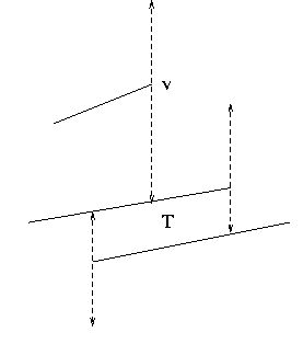
This additional work occurs when the boundary segment of a trapezoid is broken up by visibility edges from above.
|
(For convex hulls, the analogous problem was easy: two edges created per step.)
If trapezoid T is created when pi is added, then pi is incident to T.
Now consider T in TD(Ri);
what is the probability that T was created when pi was added?
That is, what is the probability that pi is a member of the S' for T?
Ri has i segments, and at most 4 of them are in S', so this probability
is <=4/i.
The expected size (number of trapezoids) of TD(Ri) is O(i+Ai2/n2), from Lemma 2 of the previous lecture, and this is independent of the choice of pi, so
Lemma 1. The expected number of trapezoids created over the course of the algorithm is sumi O(i+Ai2/n2)/i = O(n+A).
|
It may be necessary to visit trapezoids that do not meet a new segment,
in order to find those that do.
This additional work occurs when the boundary segment of a trapezoid is broken up by visibility edges from above.
|
|
|
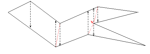
To bound the work of this kind, consider a configuration consisting
of a trapezoid with a "tail": a trapezoid together with
a visibility edge dividing its boundary.
Such a tail gives a subdivision of the boundary of the trapezoid. Since the TD is planar, the total number of such tails is O(n+A). This trap+tail configuration is determined by a set S' of at most 6 segments, just as a trapezoid is determined by at most 4 segments. |
|
When a segment traverses the graph, work is done for such a configuration if the segment meets the trapezoid, after which the configuration is gone.
So the total work for traversals is proportional to the total number of such configurations, which is O(n+A); the argument is similar as for updates, but with "6" replacing "4".
Putting these facts together, we get:
Theorem. The randomized incremental algorithm needs O(A + n log n) time to find the trapezoidal diagram of n segments with A intersecting pairs.
simple polygon, A=0
two simple polygons,
polygon with holes.
|
Connectivity can be used to reduce the search cost using "tracing": For a given random subset R of S, find the trapezoids of TD(R) that contain each endpoint of S by walking along segments of S and through TD(R) at the same time. |
|
Using tracing, connectivity information can be used to speed up the algorithm:
search takes n log*n + c log n, where:
| c | is the number of connected components, and |
|---|---|
| log*n | is the depth of log(log(...log(n))) such that the result is less than 1. |
a long-open theoretical question: can the TD be found in O(n) time?
Settled by Chazelle in 1990,
using methods inspired by those here.
Roughly,
converting from a
boundary representation, where the segments are the boundary, to an
area representation, where the trapezoids partition the interior.
Lemma 2: Tracing takes O(n) expected time when A=0 and c=1.That is, the expected total number of trapezoids touched by walking along the segments of S is O(n), or O(1) per segment.
First, an algorithm that takes advantage of this, and then the proof of the lemma.
We will change the randomized incremental algorithm somewhat,
and not maintain endpoint locations as before.
The algorithm will use the "tracing" procedure O(log*n) times:
for j with 0<=j<=log*n, let
| log(j)n | be defined by log(0)n=n, log(j)n=log(log(i-1)n). |
|---|---|
| ij | denote n/log(j)n. |
| phase j | the period of insertion of those pi with ij <= i < ij+1. |
The algorithm has about log*n phases,
with the tracing done at the end of each phase (except the last one).
The algorithm will use tracing
for S with respect to TD(Rij), for j=1..log*n.
if pi is added during phase j, so ij <= i < ij+1,
then the trapezoid of TD(Ri(j)) containing the left endpoint of pi
is known.
The usual maintenance of the trapezoid containing pi need only be done for TD(Rk), where ij < k < i.
These are the only changes.
For a given segment pi added during the first phase, the expected work for search is
for some constant C, so the total expected work for all segments in the first phase is
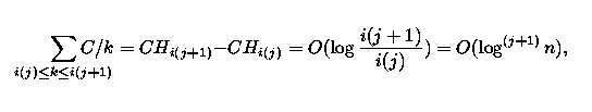
sum C/k = CHn = O(log n); 1<=k<=i
(n/log n) O(log n) = O(n).
For a segment pi added during phase j, the work for search is
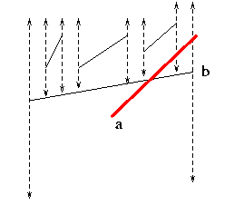
We want to show that the total number of intersections between line segments of S and trapezoids of TD(R) is expected O(n).
first observation: because A=0 here, a segment meets a trapezoid if either:
it is contained in the trapezoid, or
it crosses a visibility edge bounding the trapezoid.
The number of seg/trap meetings of the first kind is no more than n-i. So equivalently, bound the expected number of segment/visibility edge crossings.
second observation:
Pick a random element p of S.
The number of trapezoids met by all segments of S-R is n-i times
the expected number of trapezoids of TD(R) met by p.
(Here the expectation is over the random choice of p, only;
S-R denotes the set difference: members of S that are not in R.)
So:
it's enough to show that a random segment in S but not R crosses an expected O(1) visibility edges of TD(R).
Let R' denote the union of R and {p}.
Since p is a random element of S-R, and R is a random subset of S,
R' is a random subset of S, and p is a random element of R'.
V denote the visibility edges of TD(R), andThen
V' denote the visibility edges of TD(R').
V -V' is the set of visibility edges of TD(R) crossed by p, and(Here we regard two visibility edges as distinct unless they have the same starting and ending points.)
V'-V is the set of visibility edges of TD(R') incident to p.
We want to bound the expected size of V-V'.
The set V'-V is the set of visibility edges incident to p, with one endpoint or the other on p.
We have
|V-V'| + |V'| = |V'-V| + |V|,or
|V-V'| = |V'-V| + |V| - |V'|,but the size of V is 4i, and the size of V' is 4i+4, and so
|V-V'| = |V'-V| - 4,and
E|V-V'| = E|V'-V| - 4,where the expectation is with respect to the random choice of p.
The number of visibility edges of R' is 4i+4, and
each edge is incident to 2 segments, so
the expected number of edges incident to p is 2(4i+4)/(i+1) = 8.
Thus the expected number of visibility edges crossed by p is 8-4 = 4.
From the second observation above, the total number of visibility edge crossings by segments of S-R is therefore 4(n-i), and Lemma 2 follows.
A simple polygon divides the plane into two pieces, by the Jordan curve theorem. The bounded piece is the interior.
|
triangulation of a simple polygon: | a subdivision of the interior into triangles whose vertices are vertices of the polygon. |
|---|---|
| diagonal: | a line segment inside a polygon and between vertices. |
| reflex vertex: | one whose internal angle is > pi. |
| convex vertex: | one whose internal angle is <= pi. If the angle is < pi, the vertex is strictly convex. |
A TD can be used to find a triangulation in O(n) time:
A two step process:
add "local" diagonals to make x-monotone polygons;
triangulate the x-monotone polygons.
| x-monotone polygon: | a simple polygon such that the intersection of its interior with any vertical line is an interval. |
|---|
|
throw away outside trapezoids; for each inside trapezoid, check the two polygon vertices on its boundary: if they are not on the same polygon segment, draw a diagonal between them. |
|
The diagonals split the polygonal region into many polygonal regions.
The resulting polygons are x-monotone, proven as follows.
| splitter: | a vertex with two incident visibility edges in the interior. |
|---|
Two facts to prove:
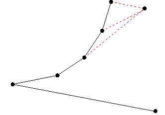
Walk from b to c. This walk begins either with x decreasing or increasing. Suppose increasing. Let v be the rightmost vertex encountered on this walk. Then v is a splitter.
Let s be a splitter vertex incident to visibility edges e and e'. Suppose e and e' are used to slice up the polygonal region.
This splits the region up into three pieces, one of which has both visibility edges as boundary. Call the latter region P'.
Let T be the trapezoid of TD(P') that is bounded by the slice. The other visibility edge bounding T is induced by a vertex that cannot be an endpoint of segments incident to s, and so there is a diagonal for s separating the two incident visibility edges.
	sort the boundary endpoints by x-coordinate.
	consider the vertices in left to right order.
	for a vertex v, add diagonals to all currently visible
		vertices to the left.
|
"It can be shown" that the currently visible vertices
to the left are as follows:
All are one chain, the top or bottom one;That is, the work is similar to finding the convex hull using the sorting-based algorithm.
|
 |
Given
a planar subdivision with n edges,build a data structure so that
given any point p, the face of the subdivision containing p can be found quickly.
The trapezoidal diagram is a refinement of the planar subdivision induced by the line segments: it's enough to locate points in TD(S).
So far, "search" has been done by maintaining the locations of endpoints. However,
This gives a planar point location data structure:
for any given point p, its location in TD(S) can be found
by tracing its location through these influence pointers.
The time required is on the order of the number of different trapezoids containing p.
For a given point p, this is expected O(log n), from Lecture 3.
This fact does not imply that the query time for the data structure is O(log n):
After the algorithm makes its random choices, an adversary picks the worst point in the plane for queries. There's no bound on how bad the query time can be.
However, two facts can be proven:
Putting these facts together, the probability that the search time fails to small is at most the sum of the failure probabilities for each class of points, or
n3/nOmega(K) = 1/nOmega(K-3)giving a small overall probability of failure.
Draw vertical lines through all segment endpoints and crossing points. Partition the resulting slabs by the segments.
There are at most {n choose 2} + 2n + 1 slabs, each cut into at most n+1 pieces by the segments, giving O(n3) pieces altogether.
Any two points in the same piece would be in the same sequence of trapezoids, and splittings of trapezoids.
This is an application of the Chernoff bound.
Let Y=sum1<=i<=n Xi, where
| Xi = |
|
Then,as before, the probability that Xi=1 is no more than 4/i, and so EY<= 4Hn.
We want to prove a bound on Prob{Y>K log n}.
Markov's inequality: For random variable X, Prob{X>K} < EX/K.
Proof: K Prob{X>K} = sumx>K K Prob{X=x} < sumx>K x Prob{X=x} <= EX.
We could apply Markov's inequality to Y,
but it's better to apply it to DY, for a value D>1 to be chosen.
Since the exponential function grows fast, a bound for DY gives
a better bound on the "tail" of Y.
We have
Prob{Y> K Hn} = Prob{DY > DK Hn} <= [EDY]/DKHn.As always, Hn is the n'th harmonic number, = sum1<=i<=n1/i.
We need to bound EDY.
Lemma 3. EDY <= g(n) == prod1<=i<=n [1 + 4D/i].
Proof: Use induction on n.
Let Y(S) denote the variable Y, for the set S.
Use conditional expectation: for random variable Z and events B and C,
EZ= E[Z|B]Prob{B} + E[Z|C]Prob{C}.
Here, the two events are:
pn is incident to the trapezoid containing the given point, or
it isn't.
With probability at most 4/i, pn is incident, and
Y(S)=1+Y(S-pn), or EDY(S) = DEDY(S-pn) < Dg(n-1) by induction
With probability at most 1, pn is not incident, and
Y(S) = Y(S-pn), or EDY(S) = EDY(S-pn) < g(n-1) by induction.
Combining conditional expectations,
EDY(S) < Dg(n-1)(4/i) + g(n-1) = g(n-1)(1+4D/i) = g(n),
and the lemma is proven.
Prob{Y> K Hn} <= EDY/DKHnand from the lemma,
EDY <= g(n) = prod1<=i<=n [1 + 4D/i].Using 1+x <= ex,
prod1<=i<=n [1 + 4D/i] <= e4DHn,and so
Prob{Y > K Hn} <= e4DHn/DKHn = e(4D-Klog D)Hn = 1/n(K(log D)-4D)
There are at most n3 classes of points, and the probability that the query time is longer than KHn is at most
e(4D-K log D)Hn,for any given point, so the probability of a query time longer than KHn anywhere is
n3/n(K(log D)-4D) = 1/nK(Log D)-4D-3.
For log D = about 1.22, the exponent is greater than 1 if K>14.
Hence: the probability that the query time exceeds 16 Hn is at most 1/n2.
So the randomized incremental algorithm yields a data structure with expected O(n+A) space, expected O(A+n log n) construction, and O(log n) query time with high probability.