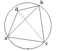
The quadrilateral acbd is convex, and has two triangulations:
T = {abc, abd}, with edge ab, the original one, and
T' = {cda, cdb}, with edge cd.
|
Suppose a triangulation is not locally Delaunay,
so some triangles abc and abd have site d inside the circumcircle of abc.
The quadrilateral acbd is convex, and has two triangulations: T = {abc, abd}, with edge ab, the original one, and |

|
Facts:
T' is Delaunay (since the other one isn't)
Angle increase: The minimum angle of T' (of the six angles) is larger than the minimum angle of T.
| Edge flip: |
The transformation of the triangulation
deleting {abc, abd} and inserting {cda, cdb},that is, swapping cd for ab. |
|---|
Note: if {a,b,c,d} are co-circular, both triangulations are Delaunay and have the same smallest angle.
...for computing a Delaunay triangulation:
	Find any triangulation of S;
	repeat
		find non-locally-Delaunay pair of triangles
		flip edge
	until the triangulation is locally Delaunay
Minimum angle of a triangulation: the smallest angle of any triangle in the triangulation
Theorem: The edge flipping algorithm terminates, and the Delaunay triangulation maximizes the minimum angle
Proof: Given a triangulation T, let
| Angle(T) = | (a1, a2,...) be the sequence of measures of angles of triangles of T, sorted into nondecreasing order. |
|---|
Suppose T is not Delaunay, and so not locally Delaunay, and so there is a triangulation T' resulting from an edge flip.
Then Angle(T') is lexicographically larger than Angle(T).
Hence if T is not Delaunay, Angle(T') is larger than Angle(T),
so the Delaunay triangulation is lexicographically maximum.
Since the number of triangulations is finite,
and each triangulation generated is distinct,
the algorithm terminates.
QED
|
The Delaunay triangulation is frequently used for
"piecewise-linear" interpolation of scattered data:
given
a set of points in the plane, and
function values at those points,
the interpolated value of the function at a point p is the value found using
linear interpolation within the triangle containing p.
That is, the graph of the interpolant function is: for each triangle abc of the Delaunay triangulation, lift it to the 3-dimensional triangle | 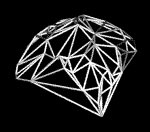 |
What is the best triangulation for this interpolation method?
It depends on the function being interpolated, which is unknown in general (except at the sites). However:
The Delaunay triangulation minimizes the maximum error when the function isf(x,y) = x2 + y2 or (x-a)2+(y-b)2for any fixed a,b.
The Delaunay triangulation minimizes the "roughness" of the interpolant, the integral of the (squared) length of the gradient.
For some functions, the Delaunay triangulation is not the best; better triangulations are often found by local improvement using edge flipping.
For a given set S of sites, the geometric graph G(S) on S has:
the sites as vertices, and
has all edges {a,b} between sites a and b,
with weight equal to the distance between the a and b.
For a given set S, the following undirected graphs have vertex set S, and weighted edges {a,b}, for a,b in S, with weight d(a,b). Let:
| G(S) | have all edges. | |
|---|---|---|
| RNG(S) | , the Relative Neighborhood Graph, have edges between sites a and b when no third site is closer to a and to b than d(a,b). That is, the shaded lune in the figure is empty. |  |
| GG(S) | , the Gabriel graph, have edges between sites a and b when no site is closer than a and b to the midpoint of segment ab. The shaded circle is empty. |  |
| MST(S) | be the minimum spanning tree of G(S). |
Fact: the edge sets of these graphs haveMST(S) subset RNG(S) subset GG(S) subset DG(S) subset G(S).
Proof sketch: Recall that an edge e of a graph is in no MST of the graph if e is the heaviest edge in some cycle of the graph. If an edge {a,b} is not in RNG(S) due to some site c, then {a,b} is heaviest in the cycle a-b-c-a. For the rest, proof by picture. QED
Given a graph G and parameter t, a t-spanner G' of G has the same vertices, and perhaps fewer edges, but the distance between a and b in G' with a factor of t of the distance between a and b in G.
Fact: DG(S) is a 2.43-spanner of G(S).
Proof omitted.
Some algorithms
Given sets L and R, S= L union R, separated by a vertical line, and their triangulations DG(L) and DG(R), compute DG(S).
There are RR edges, LL edges, and cross edges.
All new Delaunay edges in the merge are cross edges: if an RR edge is Delaunay now, it was before.
Some triangles of DG(L) are deleted: those with circumcircles
containing points of R.
...and symmetrically for DG(R).
The cross edges are ordered along the split line, and consecutive edges share a vertex.
The cross edges are built from bottom to top, starting from a cross edge that is a convex hull edge.
|
Conceptually, maintain an empty disk on the current cross edge {a,b}, pushing it up, but keeping a and b on the bounding circle. The first site this "rising bubble" hits gives the next cross edge. That site is on an edge incident to a or b. To find it,
  walk around
  the edges incident to a, deleting those bounding
  triangles conflicting with b.
  Find the first edge {a,a'} not deleted.

  Similarly walk around the edges incident to b,
  finding edge {b,b'}.

  Either b or b' is hit first by the
  "rising bubble", yielding the next cross
  edge {a,b'} or {a',b}.
Since O(n) work is done in the merge, O(n log n) is needed overall. Dwyer has shown that O(n log log n) is needed for points uniform in the square, using bucketing. | 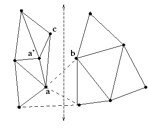 |
There are at least four viewpoints of the sweep algorithm.
|
When viewed as a Delaunay triangulation algorithm: Sweep a vertical line from left to right.
For a point p on the sweep line, is empty: has no sites inside; S(p): the sites on the tangent empty circle of p. The points on the sweep form equivalence classes based on S(p). | 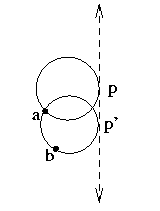 |
Intervals of points have the same S(p) with |S(p)|=1, separated by points with |S(p)|=2, corresponding to Delaunay edges.
Suppose the circle event has S(p)={a,b,c}, |
|
|
At a site event, suppose site a is met by the sweep, in an interval labeled by {b}, and bounded by {b,c} and {b,d} Then a new interval, labeled by {a} and bounded by {a,b} on both sides, will be seen. Output Delaunay edge ab. Check for circle events for {a,b} and {b,c}, and for {a,b} and {b,d}. Some scheduled circle events will not actually occur: for example, if a site event splits an interval, that interval cannot shrink to a point. |
|
Such "false alarm" events can be detected and removed when real events occur, and there are a bounded number of them.
We next turn to the problem of computing convex hulls of point sets in higher dimensions; to do this, many basic facts about convex sets must be known. While actually proving these facts rigorously is a course in itself, proving some of them will motivate introducing some machinery that is useful in its own right.
Some of the facts needed are these:
As an example of the last fact: recall that the Voronoi region of a site is a polygon, if bounded: the intersection of all the halfspaces containing the site and bounded by the perpendicular bisectors of the site and other sites.
But it is also the convex hull of its vertices. This fact holds for any bounded convex polyhedral sets. They are both: the convex hulls of their vertices, and the intersection of the halfspaces bounded by their facets (edges in 2d).
The convex hull problem is to convert between these presentations: given a set S of points, find the halfspaces whose intersection is conv(S).
We'll next review basic ideas of convexity, then state and/or prove some basic facts about convex sets.
Let S be a set of points, and zp a coefficient for each point p in S. Then a point of the form
sump in S zp pis a combination of the points of S, of the kind shown in the table, depending on the properties of the coefficients. The table also gives the name of the corresponding sets closed under such combination, and the closure operation applied to the set.
| combination | conditions on zp | closed set | closure | |
|---|---|---|---|---|
| linear | none | linear subspace | span(S) | |
| positive, conical | zp >= 0 | cone | cone(S) | |
| affine | sump in S zp = 1 | affine subspace, flat | aff(S) | |
| convex | zp >= 0, sump in S zp = 1 | convex set | conv(S) | |
Note that a convex combination is affine and positive: conv(S) is the intersection of cone(S) with aff(S).
For example, three collinear points are affinely dependent.
There are similar ideas of independence for the other forms:
linear independence for linear combinations,dim(P) : ==dim(aff(P)) == one less than the size of the largest affinely independent set in P.
"in convex position" for convex combinations.
Also, dim(P) == the linear dimension of P-p, for any point p in P. That is, translate aff(P) to contain the origin; the resulting linear subspace has dimension dim(P).
Two distinct points S;
| span(S) | is a plane through the origin, |
| cone(S) | is a planar "wedge" with apex at the origin, |
| aff(S) | is the line through the points, and |
| conv(S) | is the line segment between the points. |
Three distinct points:
| span(S) | is a 3-dimensional hyperplane through the origin. |
| cone(S) | is a cone with apex at the origin, with three sides. |
| aff(S) | is the plane through the points, and |
| conv(S) | is the triangle with the three points as vertices. |
A few more definitions, for sets P and Q:
| relint(P) | : (mentioned in Lecture 5) the relative interior of P, relint(P), is the interior of P, as a subset of aff(P), |
|---|---|
| P+Q | : for sets P and Q, the Minkowski sum P+Q is the set {p+q | p in P, q in Q}. |
| simplex | : conv(S) for an affinely independent set S. |
| P(H): | for a set H of closed halfspaces, P(H) is the intersection of the halfspaces in H. |
|---|
Since each halfspace is convex, and the intersection of convex sets is convex, P(H) is convex: a polyhedral set or convex polyhedron.
However, not all P(H) can be described as conv(S) for some finite point set S. For example, unbounded Voronoi regions cannot be.
This makes the connections between the H-polyhedra and V-polyhedra messy; the correct relation is that every P(H) can be written as conv(S)+cone(Y), for some sets S and Y.
Rather than deal with such awkwardness, it's better to move to cones.