Sampling and Sketching for `M`-estimators
Ken Clarkson
IBM Research, Almaden
Joint with David Woodruff
IBM Research, Almaden
Least-squares regression
- Input is `n` points in `d+1` dimensions
- Points have the form `(A_i,b_i)`,
where:
- `A` is an `n \times d` matrix
- `A_i\in \reals^d` is row `i` of a matrix `A`
- `b\in\reals^n` is a column vector
-
Regression [G95][L05]: find
$$
\min_{x\in\reals^d}\norm{Ax-b}_2
$$
- `r\equiv Ax-b` is the residual
- `\norm{r}_2 = \sqrt{\sum_i r_i^2}`, the length of `r`


Least-squares is not very robust
`M`-estimators


- `M`-estimators: min `\norm{r}_G\equiv \sum_i G(r_i)`,
for some function `G`- `G(z) = z^2`: `\ell_2^2` least-squares
- `G(z) = |z|`: `\ell_1` regression
- `G(z) = \begin{cases}
z^2/2\tau & z \le \tau
\\ |z| - \tau/2& z\ge \tau
\end{cases}`
- ...the Huber estimator [H64]
- Robust, yet smooth
- Tukey: even more robust
Results
- `\nnz{A} \equiv ` number of non-zeros of `A`
- `\epsilon \equiv` error parameter
- Huber:
`\qquad O(\nnz{A}\log n))+\poly(\eps^{-1}d \log n)` time
for any given `\epsilon>0` - For nice functions `G(z)`, and fixed large enough `\eps`:
- Reduce problem size: compress `A` and `b`, the same for all `G`
- Find approximate solution in `\qquad O(\nnz{A}) + \poly(d\log n)` time,
convex `G`
Seek `\hat x` with small relative error: $$\norm{A\hat x - b}_G \le (1+\epsilon)\min_{x\in\reals^d} \norm{Ax - b}_G$$
"Nice" `G`
- Functions `G(x)` that are
- even: `G(x) = G(-x)`
- monotone nondecreasing in `|x|`
- for `|a|\ge |b|`, $$\frac{|a|}{|b|}C_G \le \frac{G(a)}{G(b)} \le \frac{a^2}{b^2}$$ for some `C_G > 0`
- Upper bound required for `\norm{\,}_G` to be sketchable [BO10]
- Need not be:
- Convex
- Smooth
- Tukey is not nice, but a close variant is
( `\norm{\,}_G` and norms )
- Despite the notation, `\norm{\,}_G` is not a norm
- But:
- For many `G` proposed, `\sqrt{\norm{\,}_G}` satisfies the triangle inequality
- For nice `G` and `\kappa\ge 1`, $$\sqrt{\norm{x}_G}\sqrt{\kappa C_M} \le \sqrt{\norm{\kappa x}_G}\le \kappa \sqrt{\norm{x}_G}$$
- That is, `\sqrt{\norm{\,}_G}` is "scale insensitive"
- vs. e.g. `\norm{\kappa x}_2 = |\kappa|\norm{x}_2`
Sketching `A`
- We apply sketching to regression (including here also row sampling)
- Sketch of `A` is `SA`, sketch of `b` is `Sb`
- `S` is a matrix with `m\ll n` rows
- `m=O(d)` or `O(d^2)`, usually
- `SA` reduces the number of points (rows)
- `A\hat S` reduces the dimension (number of columns), for appropriate `\hat S`

Using `SA` for regression
- `S` is an embedding, preserving lengths
- This is basically the same as $$ \norm{S(Ax-b)} \approx \norm{Ax-b} \text{ for all } x $$
- If `\tilde x` is such that
`\qquad` `\norm{SA\tilde x - Sb} = \norm{S(A\tilde x-b)}\text{ is minimum}`
then
`\qquad` `\norm{A\tilde x - b}\text{ is small.}`
The key property: `\norm{SAx} \approx \norm{Ax} \text{ for all } x`
For regression, only need "lopsided" embedding:
$$\norm{SAx} \ge (1-\eps) \norm{Ax} \text{ for all } x$$
and
$$\norm{SAx^*} \le (1+\eps)\norm{Ax^*}$$
Sketching (in general)
- A random distribution over `S`, so that for given `A`, embedding holds w.h.p.
- For example:
- (Non-uniform) row samples
- JL, Fast JL
- All entries of `S` i.i.d.
- Here, for "nice" `M`-estimators, `S` such that:
- `S` and `SA` can be computed in `O(\nnz{A}\log n)` time
- vs. `O(mnd)` or `O(dn\log n)`
- `S` and `SA` can be computed in `O(\nnz{A}\log n)` time
- Typical proof technique:
- Show that `\norm{SAx}\approx \norm{Ax}` for fixed `x` with high probability
- Apply union bound for `x\in {\cal N}` an `\epsilon`-net
Outline
- Huber: we use `S` that implements row sampling
- Sketching for nice `\norm{\,}_G`: we extend Sparse Embeddings (good for `\ell_2`) with a family of uniform samples
Sampling for embedding
- Uniform sampling of rows by itself does not give an embedding
- Need non-uniform sampling: pick row `i` ind. with probability `q_i`
- Apply weight `1/q_i` appropriately
- Number of rows picked is random
- Row of `S` is a multiple of `e_i`
- For `\ell_p`, there are `q_i` so that this yields an embedding
- `\sum_i q_i = \E[\text{num rows}] = \poly(d/\eps)`
- For `\ell_2`, from the leverage scores
- For general `p`, `p`'th power of norm of row `i` of well-conditioned basis for `A`
- For any `p`, find `q_i` in `O(\nnz{A}\log n) + \poly(d/\eps)` time [CW13]
Sampling for Huber embedding
- Huber is roughly `\ell_2^2` for small values, `\ell_1` for large
- We show that a combination of `q_i`s for `\ell_2` and `\ell_1` yields useful sampling probabilities
- But: `\sum_i q_i = \E[\text{num rows}] = \Theta^*(\sqrt{n})`
- We recurse `n\rightarrow\sqrt{n}\rightarrow n^{1/4}\rightarrow\cdots`
- Until general convex programming can be applied
Sketching for nice `\norm{\,}_G`: sparse embeddings
- A construction that yields an embedding for `\ell_2`
- Adaptation of
CountSketchfrom streaming algorithms- [CW13,NN13,MM13]
- `S` looks like:
$\qquad\qquad\left[\begin{matrix} 0 & -1 & 0 & 0 & +1 & 0 \\ +1 & 0 & 0 & +1 & 0 & 0 \\ 0 & 0 & +1 & 0 & 0 & -1 \\ 0 & 0 & 0 & 0 & 0 & 0 \end{matrix} \right]$
- One random `\pm 1` per column
- Row `a_{i:}` of `A` contributes `\pm a_{i:}` to one row of `SA`
- `m=\tO(d^2)`
Sparse embeddings, more


- For `y=Ax`, each row of sparse embedding `S`:
- Collects a subset of entries of `y` (into a "bucket")
- Applies random signs
- Adds
- Result is `\norm{Sy}^2 \approx \norm{y}_2^2`:
- Each bucket squared `\approx` squared norm of its entries
- Splitting into buckets separates big entries
- Smaller variance
Sketching `M`-estimators
- How to sketch so that `\norm{Sy}_G \approx \norm{y}_G`?
- Suppose `G(x) = |x|`, so `\norm{y}_G= \sum_i |y_i| = \norm{y}_1`
- Consider two one-row sketches:
- Uniform sampling: pick random `i^*`, `S_{1i} \gets\begin{cases} n & i=i^*\\0 & i\ne i^*\end{cases}`
- `\ell_2` sketching: `\hat S = (\pm 1,\pm 1,\ldots,\pm 1)`
- `\norm{Sy}_G = G(Sy) = |Sy|`, since `S` has one row
Uniform vs. `\ell_2` sketches, for `\ell_1`
| Sampling `S` | `\ell_2` Sketching `\hat S` | |
| General `y` | `\E[|Sy|] = \norm{y}_1` | `\E[|\hat Sy|] \approx \norm{y}_2` |
| `e_1=(1,0,\ldots,0)` | `\Var[|Se_1|] = n-1` | `|\hat Se_1| = 1 =\norm{e_1}_1` |
| `\bfone=(1,1,\ldots 1)/n` | `|S\bfone| = 1` | `\E[|\hat S\bfone|] \approx 1/\sqrt{n} \ll 1 = \norm{\bfone}_1` |
`M`-sketches
`S \gets \left[ \begin{matrix}S_0T_0 \\ S_1T_1 \\\vdots\\ S_{\log n}T_{\log n}\end{matrix}\right]`
- Combine sampling and sparse embedding
- [VZ12] earthmover, [CW15] `M`-estimators
- Each `S_h` is a sparse embedding matrix
- Each `T_h` samples about `n/b^h` entries, then multiplies by `b^h`
- For parameter `b`
- Result: `\norm{SAx}_{w, G} \approx \norm{Ax}_G`
- A lopsided embedding for constant approximation with constant prob.
- Where `\norm{y}_{w,G} = \sum_i w_i G(y_i)` for weight vector `w`
- Claim true for any given `G`
`M`-sketch analysis
- For given `y` with `\norm{y}_G=1`, define weight classes
`W_j \equiv \{ G(y_i) \mid 2^{-j-1}\le G(y_i)\le 2^{-j} \}` - For suitable `b` and other parameters, there is `h_j` such that with high enough probability:
- For `h\approx h_j`, the entries of `T_h y` from `W_j` are in separate CountSketch buckets
- Contributing about `\norm{W_j}_G` to `\norm{y}_G`
- And for `|W_j|` large, this concentrates
- For `h \gg h_j`, there are no entries in `T_hy` from `W_j`
- For `h \ll h_j`, the entries of `T_h y` from `W_j` appear many-per-bucket
- And contribute roughly `G(\norm{W_j}_2)` to `\norm{y}_G`
- For `h\approx h_j`, the entries of `T_h y` from `W_j` are in separate CountSketch buckets
- If `G` is fast growing, need to "clip" small buckets (Ky Fan vector norm)
A Matlab Version
Just to show it's not very complicated:
   function [ S ] = M_sketch(n, d, b)
    S.num_buckets = 1+floor(b*d*(1+log(n)));
    S.level = 1 + random('geo', 1-1/b, n);
    S.sign_flip = randi(2, n)*2 - 3;
    S.hash = randi(S.num_buckets, n);
   end

   function [ Sy ] = M_sketch_apply( S, y)
    Sy = zeros(max(level), S.num_buckets);
    for i=1:length(y)
        li = S.level(i);
	hi = S.hash(i);
        Sy(li, hi) = Sy(li, hi) + y(i)*S.sign_flip(i);
    end;
   end

   function [ est ] = M_sketch_eval( Sy, b, G )
    est = 0;
    for i=1:size(Sy,1)
	est = est + (b^(i-1))*sum(G(Sy(i,:)));
   end
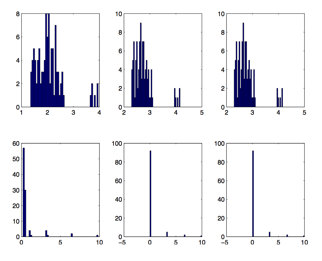
Experiments
- For `\bfone=(1,1,\ldots 1)/n` and `\bfone+10e_1`:
- Estimate `\norm{y}` using sketch
- Compare to actual norm
- `n=1e6`
- Sketch dim `\approx` 1e4
| Vector | `\ell_1` | `\ell_2^2` | Huber |
| `\bfone=(1,1,\ldots 1)/n` | 1 | `1/n` | `1/n` |
| `\bfone + 10e_1` | `11` | `\approx 100` | `\approx 10` |
Results
- Histogram of `\log_2(\text{Est/Act})`
- `\bfone` above, `\bfone+10e_1` below