Self-Improving Algorithms
`\qquad\quad`Ken Clarkson
Joint with
Nir Ailon, Bernard Chazelle, Ding Liu, C. Seshadhri, Wolfgang Mulzer
IBM Almaden,
Princeton Univ., both
(at the time, before 2013)


Machine Learning
Risk minimization
The setup:
The goal: use samples `z_k` to approximately find `\argmin_{c\in C} \E_{z\sim\cD}[\ell(c,z)]`
For example, classification:- Training samples `z_1,z_2,\ldots`, where `z_k \sim \cD`
- Concept space `C`
- Loss function `\ell(c, z)\rightarrow \R^+` for `c\in C`, `z\sim\cD`
- Risk of `c\in C` is `\E_{z\sim\cD}[\ell(c,z)]`
The goal: use samples `z_k` to approximately find `\argmin_{c\in C} \E_{z\sim\cD}[\ell(c,z)]`
- Also given: function `f(z)`
- `C` is a set of functions on `z`
- Loss `\ell(c,z)` is the expense if `c(z)\ne f(z)`
Here:
- Also given: function `f(z)`
- `C` is a set of algorithms with output `c(z) = f(z)`
- Loss `\ell(c,z)` is the running time of algorithm `c` on `z`
So: for a given task and distribution over inputs, learn to run fast
Finding `\argmin`
Or at least, `\mathrm{arggood}`
- Empirical risk minimization: minimize
$$\sum_k \ell(c, z_k)\approx \E_\cD[\ell(c,z)]$$ can be helpful [GR16], but not always- May be too hard: no gradient in `C` space, etc.
- Table lookup might win on training samples
- Our strategy:
- Find lower bound for best running time `\min_{c\in C}\E_\cD[\ell(c,z)]`
- Construct algorithm that provably achieves it
Need conditions on `C` and `\cD` to make these possible
Tasks


Categories of `f` in this work:
- Sorting
- Delaunay triangulations
- Convex hulls (upper hull)
- Coordinate-wise maxima
Each input `z=(x_1,\ldots,x_n)`, where
`x_i` are all real values, or
`x_i` are all points in the plane
Conditions on outputs
- Combinatorial objects
- Includes certificates that allow verification in `O(n)` time
e.g. for maxima:- sequence of maxima, and
- for each dominated point, a witness point dominating it
Particular proof structure is a particular way
to model work that a correct algorithm must do
Conditions on algorithms
- Not too much space or training samples
- Correct for all possible inputs
- Work done is `\Omega(n)`
- Key operation on data is comparisons
- Output determined by `\mathrm{compseq}(c,z)`, the sequence of comparisons
- `\textrm{Work} = \Omega(n+|\mathrm{compseq}(c,z)|)`
- Broad category of possible comparisons
- Use "natural" comparisons in geometric setting
A comparison yields at most one bit of information
Entropy lower bounds
- `f(z)` is a random variable, since `z` is
- `f(z) = ` output of `c` using `\mathrm{compseq}(c,z)`
- So `\E[|\mathrm{compseq}(c,z)|] \ge H(f(z))`, the entropy of the output
- Shannon
- Work lower bound is `\Omega(n + H(f(z)))`
Meeting the entropy lower bound (prior work)
A classical example fits these conditions:entropy-optimal search trees
- Given some sorted list `L` of values
- Function `f(z)`:
`\qquad` Real value `z\rightarrow` `j`-th interval containing `z` - `\Omega(1+H(f(z)))` comparisons
- Achievable [M75] via entropy-optimal trees `T`

Conditions on `\cD`
- We require `\cD = \prod_i \cD_i`
- For `z=(x_1, x_2,\ldots,x_n)`, `x_i \sim \cD_i`
- Each `x_i` independent of the others
- Not all identical
- Distributions `\cD_i` are:
- Arbitrary
- Unknown
- Discrete and/or continuous
- Algorithms here use polynomial space
- There exist `\cD` (without independence) such that
`\exp(\Omega(n))` space is needed for time `O(n + H(f_S(z)))`
Results: meeting the entropy lower bounds
Under these conditions: comparison-based algorithms, proof-carrying output, product distributions...
- Algorithms doing `O(n + H(f(z)))` comparisons and work
- (plus `O(n\log\log n)` for convex hull)
- `O(n^2)` training instances `z_k`
- `O(n^2)` space
- For given `\alpha \in (0,1]`,
- `O(n + H(f(z)))/\alpha` comparisons
- `O(n^{1+\alpha})` training instances `z_k`
- `O(n^{1+\alpha} \log n)` space
- Tradeoff is tight, even for sorting
Sorting : The Typical Set `V`
- Sorting algorithm uses a set `V` of "typical" values
- `V` is built using training samples, as follows:
- Let `W := \mathrm{sort}(z_1 \cup z_2 \cup ... \cup z_{\lambda})`
- `\lambda := K \log n`, for a constant `K`
- Let `V:=` the list of every `\lambda`-th value of `W`
- `v_i = w_{\lambda i}`
- `|V| = n`
- `V` represents the overall distribution of `z`
- We expect about one value from `z` in each interval `[v_j, v_{j+1})`

Sorting : Search Trees `T_i` on `V`
To use `V`, we build, for each `x_i`,an entropy-optimal search tree `T_i` over `V`
As above:
- Search random variable is bucket index `b_i:= j` when `x_i\in [v_j, v_{j+1})`
- The search cost is `1+H(b_i)`
- Additional training instances are used to build `T_i`
Sorting : The Algorithm
- After training, the algorithm is:
- Expected `O(1)` work/bucket, so total over buckets is `O(n)`
- Searches are entropy-optimal
- So we're done, right?
For each `i=1..n`:
`\qquad` locate `x_i` in the buckets using `T_i`
For each bucket:
`\qquad` sort the set of values falling in each bucket
`\qquad` locate `x_i` in the buckets using `T_i`
For each bucket:
`\qquad` sort the set of values falling in each bucket
Analysis
- We're not quite done
- Although the `T_i` are individually optimal,
it hasn't been shown that their cost is small - It remains to show that `\sum_i O(1+H(b_i)) = O(n+H(f_S(z)))`
Analysis via Coding
- Independence `\implies \sum_i O(1+ H(b_i)) = O(n + H(b))`,
`\qquad` where `b= (b_1,...,b_n)` - Note that `b` can be computed from `f_S(z)`,
using `O(n)` additional comparisons:Sort the values `x_i` using `f_S(z)`
Merge that sorted list with `V`, with `O(n)` comparisons
Read off bucket assignments from merged list
So `b` can be encoded using
- An encoding of `f_S(z)`, plus
- `O(n)` bits for the comparisons
`H(b)\le` encoding cost ` = O(n+H(f_S(z)))`
Search work ` = O(n+H(b)) = O(n+H(f_S(z)))`
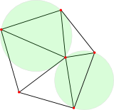
Delaunay Triangulations
- Given a set `z` of points,
its Delaunay triangulation `f_T(z)` is a planar subdivision whose vertices are the points in `z` - If a triangle `T` has:
- Vertices from `z`, and
- No points of `z` in its circumscribed disk
- Then `T` is a Delaunay triangle, with a Delaunay disk
- A Delaunay triangulation comprises all such Delaunay triangles
- (Ignoring the unbounded parts)
Sorting vs. Triangulation
- Delaunay triangulation is like sorting, only more complicated
- Actually, sorting can be reduced to Delaunay triangulation
- We can view sorting as:
`\qquad` find all open intervals `(x_i, x_{i'})` containing no `x_{i''}`, all from `z` - We can view finding the Delaunay triangulation as:
`\qquad` find all Delaunay disks - Algorithm and analysis for triangulation generalizes that for sorting
Sorting::Delaunay as...
| Sorting | Delaunay Triangulation |
|---|---|
| Intervals `(x_i, x_{i'})` containing no values of `z` | Delaunay disks |
| Typical set `V` | Range space `\epsilon`-net `V` [MSW90, CV07], Ranges are disks, `\epsilon = 1/n` |
| `\log n` training sample points per bucket | `\log n` training sample points per disk |
| Expect `O(1)` values of `z` in each bucket | Expect `O(1)` points in each D. disk of `V` |
| Entropy-optimal search trees `T_i` | Entropy-optimal planar point location `T_i` [AMMW07] |
| Sorted within each bucket yields `f_S(V \cup z)` in `O(n)` |
Triangulated within each small region yields `f_T(V \cup z)` in `O(n)` |
| Removal of `V` from sorted `V \cup z` (trivial) | Build `f_T(z)` from `f_T(V \cup z)` [ChDHMST02] |
| In analysis: merge of `f_S(V)` and `f_S(z)` to get `f_S(V\cup z)` | In analysis: merge of `f_T(V)` and `f_T(z)` to get `f_T(V\cup z)` [Ch92] |
| In analysis: recover buckets `b_i` from sorted `f_S(V \cup z)` (trivial) | In analysis: recover triangles `b_i` in `f_T(z)` from `f_T(V \cup z)` |
Why the "easier" problems are hard
- Delaunay triangulation includes convex hull
- Hard to acount for work in proving points not on hull
- Non-upper-hull `x_j, j=n/2+1,\ldots, n` easily proven by `\overline{x_1 x_{n/2}}`
- Don't need to sort them
- When points close to hull, have to sort
- When `x_1,x_{n/2}` equally likely at two positions,
none/some/all remain on upper hull

`x_1,\ldots,x_{n/2}` are fixed (singleton distributions)

`x_1,\ldots,x_{n/2}` are fixed (singleton distributions)

`x_1,\ldots,x_{n/2}` are fixed (singleton distributions)
Algorithms for maxima and hull


- Both build set `V` (of horizontal coords of `x_i`s) and trees `T_i` for each `\cD_i` or related distributions
- Strategy: search for each point `x_i` only as far down as is necessary for correctness
- Maxima: sweep from right to left, maintaining leftmost maximum
- Traverse `T_i` for each `x_i` that is
not yet out, and might be rightmost not-swept
- Traverse `T_i` for each `x_i` that is
- Hull: also build a polygonal curve so that any supporting line has little mass above it
- Use that curve to help find certificates
Concluding Remarks
- 😤 The results are pleasingly tight
- 😥 😱 Not enough bang for buck: all that work for a `\log` factor
- 😊 Novelty for me: the coding arguments
- 😲 Are there stronger conditions that imply cheaper algorithms?
- 😲 Are there broader conditions that allow interesting results?
- `\qquad` Without full independence of each `x_i`, for example