Geometric Optimization
and/or/in
Machine Learning, and Related Topics
Ken Clarkson
IBM Almaden Research
CG v. ML
| VC dimension | VC dimension |
| JL/sketches | JL/hash kernels |
| iterative re-weighting | multiplicative weights |
| "random sampling" | sample compression |
| coresets | sparse greedy approximation |
| backwards analysis | deletion estimates |
| surface reconstruction | manifold inference |
| `k`-NN graph | `k`-NN graph |
| polytope approximation | non-negative matrix factorization |
| Minimum Enclosing Ball | Support Vector Data Description |
| Polytope distance | Training linear classifiers |
| low-to-medium dimension | high dimension |
| approximation error | classification error (risk) |
| run-time w.r.t. `n` and `\epsilon` | run-time w.r.t. risk |
Outline
- Some geometric problems, algorithms, analysis
- Approximation algorithms
- First order methods (no second derivatives)
- Analysis using on-line convex optimization formalism
- But the problems and algorithms are not on-line
- Fast randomized approximate evaluation of dot products
- Alternatives to JL
- Matrix Bernstein and applications
- A primal-dual algorithm
- (Significant) algorithmic results are joint with Elad Hazan and David Woodruff
Some Geometric Optimization Problems
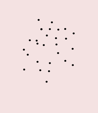
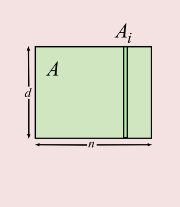
- Throughout, a set of `n` points in `d` dimensions, with norms `\le 1`
- In `A`, a `d\times n` matrix
- Column `i` of `A` is `A_i=A_{:i}`, row `j` is `A_{j:}`
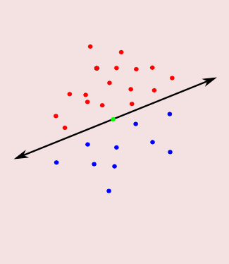
- Perceptrons: points are red or blue, split colors by a hyperplane
- A flavor of linear programming, or quadratic (when maximizing margin)
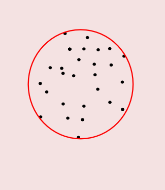
- Minimum Enclosing Ball (MEB): find the smallest ball containing the points
- A flavor of quadratic programming
Quadratic Programming in the Simplex
- MEB, Perceptron, etc. are instances of
$$\min_{p\in\Delta_n} \norm{Ap}^2 + p^\top b,$$ where- `\Delta\equiv \Delta_n \equiv` the unit simplex `\equiv \{p\in\reals^n \mid \sum_i p(i) = 1, p(i)\ge 0\}`
- `b \in \reals^n`
- Objective function is convex, `A\!\Delta` is the convex hull of input points
- `L_2`-SVM is also QP in the simplex
- A linear classifier model, where off-side points are allowed but penalized
QP in the Simplex, Weak Duality
- Why are these problems QP?
- Two observations:
- `\norm{y}^2\ge 0`, for a vector `y`
- `\min_{p\in\Delta_n} p^\top y = \min_{i\in [n]} y(i)`
- For `v,x\in\reals^d`:
$$\norm{v-x}^2 \ge 0$$ - So:
$$\norm{v}^2 \ge 2x^\top v - \norm{x}^2$$ - Letting `v\leftarrow Ap`:
$$\norm{ \color{green}{Ap} }^2 \ge 2x^\top \color{green}{Ap} - \norm{x}^2$$ - Add `p^\top b` to both sides:
$$\norm{Ap}^2 \color{green}{+ p^\top b} \ge 2x^\top Ap - \norm{x}^2 \color{green}{+ p^\top b} $$ - Taking `\min` on both sides:
$$\color{green}{\min_{p\in \Delta}}\norm{Ap}^2 + p^\top b \ge \color{green}{\min_{p\in \Delta}}2x^\top Ap - \norm{x}^2 + p^\top b $$ - Since this holds for all `x`, we have:
$$\min_{p\in \Delta} \norm{Ap}^2 + p^\top b \ge \color{green}{\max_{x\in\reals^d}} \min_{p\in \Delta} 2x^\top Ap - \norm{x}^2 + p^\top b$$ - By Observation (2):
$$\min_{p\in \Delta} \norm{Ap}^2 + p^\top b \ge \max_{x\in\reals^d} \color{green}{\min_{i\in [n]}} 2x^\top \color{green}{A_i} - \norm{x}^2 + \color{green}{b_i}$$ - This is the weak duality relation between two optimization problems
QP `\rightarrow` Perceptron
- Duality, again:
$$\min_{p\in \Delta} \norm{Ap}^2 + p^\top b \ge \max_{x\in\reals^d} \min_{i\in [n]} 2x^\top A_i - \norm{x}^2 + b_i$$ - When `b=0`, LHS is "shortest vector in a polytope"
- RHS: $$\max_{x\in\reals^d} \min_{i\in [n]} 2x^\top A_i - \norm{x}^2$$
- Letting `x = \beta y`, for `\beta\ge 0`: $$\max_{y\in\reals^d} \max_{\beta\ge 0} \min_{i\in [n]} 2\beta y^\top A_i - \beta^2\norm{y}^2$$
- When all `y^\top A_i \ge 0`: $$\max_{y\in\reals^d} \min_{i\in [n]} (y^\top A_i)^2/\norm{y}^2$$
- So opt. maximizes the min distance of `A_i` to hyperplane
- cf. [GJ] Polytope distance
QP `\rightarrow` MEB
- Duality, again:
$$\min_{p\in \Delta} \norm{Ap}^2 + p^\top b \ge \max_{x\in\reals^d} \min_{i\in [n]} 2x^\top A_i - \norm{x}^2 + b_i$$ - When `b_i \equiv -\norm{A_i}^2`, $$2x^\top A_i - \norm{x}^2 -\norm{A_i}^2 = -\norm{x-A_i}^2$$
- The weak duality relation becomes
$$\max_{p\in\Delta} -(\norm{Ap}^2 + p^\top b) \le \min_{x\in\reals^d} \max_{i\in[n]} \norm{x-A_i}^2 = R_{A}^2$$
- `R_A\equiv` MEB radius of `A`
A Simple Algorithm for MEB
`x_1 \leftarrow A_1`
for `t=1,\ldots,T`:
`i_t \leftarrow \argmax_{i\in[n]} \norm{x_t - A_i}` // Farthest from current
`x_{t+1} \leftarrow \sum_{\tau\in [t]} A_{i_\tau}/t` // Centroid of farthest points
return `\overline{x}\leftarrow \sum_{t\in [T]} x_t/T`.
for `t=1,\ldots,T`:
`i_t \leftarrow \argmax_{i\in[n]} \norm{x_t - A_i}` // Farthest from current
`x_{t+1} \leftarrow \sum_{\tau\in [t]} A_{i_\tau}/t` // Centroid of farthest points
return `\overline{x}\leftarrow \sum_{t\in [T]} x_t/T`.
The Frank-Wolfe algorithm, more or less.
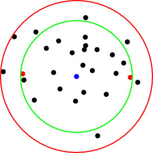
Demo
- `\color{red}{x_t}`
- `\color{green}{\overline{x}}`
- `\color{blue}{A_{i_\tau}}` for some `\tau`
Analysis: Regret
- Each iteration, define "cost" `c_t(x)\equiv \norm{x-A_{i_t}}^2`, so
`c_t(x_t) = \max_{i\in[n]} \norm{x_t - A_i}^2 \ge R_A^2` - The regret of `\{x_t\}_{t\in[T]}` is `\sum_{t\in[T]} c_t(x_t) - \sum_{t\in[T]} c_t(x_*)`
- `x_*` minimizes `\sum_{t\in [T]} c_t(x)`
- "Excess" cost of the sequence `\{x_t\}_{t\in[T]}` for `A'\equiv \{A_{i_t}|t\in[T]\}`
- Here:
- `x_*= x_{T+1}` is the centroid of `A'`
- Each `x_{t+1}` minimizes total cost against all `A_{i_\tau}` for `\tau\in[t]`
- Fact: here the regret is `O(\log T)`
Analysis, using Regret
`\eqalign{ R_{A'}^2 & = \min_x \max_{t\in [T]} c_t(x) \\ & \ge \min_x \frac{1}{T}\sum_{t \in [T]} c_t(x) & \quad \textrm{(max }\ge \textrm{ average)} \\ & \ge \frac{1}{T}\sum_{t \in [T]} c_t(x_t) - O(\log T)/T & \quad \textrm{(regret bound)} \\ & \ge \frac{1}{T}\sum_{t\in [T]} \norm{x_t - A_i}^2 - O(\log T)/T & \quad \textrm{(for each } i\in[n]) \\ & \ge \norm{\overline{x} - A_i}^2 - O(\log T)/T & \quad \textrm{(convexity of } \norm{x-A_i}^2) \\ }`Analysis, Wrapup
- `R_A^2 \ge R_{A'}^2 \ge \norm{\overline{x} - A_i}^2 - O(\log T)/T`, for every `i\in[n]`
- So `R_A(\overline{x})^2 \le R_{A}^2 + O(\log T)/T`
- Error `\epsilon` for `T=O(\log(1/\epsilon)/\epsilon)`
Related Work: Coresets,
Low-Rank Approximation
- Coresets: small subsets of input that specify approximate solutions
- For `\epsilon`-coreset `C`, `A\subset (1+\epsilon)\textrm{MEB}(C)`
- A variety of applications since introduced about a decade ago
- The set `\{A_1\}\cup A'` is a coreset
Coresets, via Regret
- The set `\{A_1\}\cup A'`, plus the algorithm, specifies approx. center $\overline{x}$
- The algorithm runs the same on `\{A_1\}\cup A'` as on `A`
- Also: by regret,
`\eqalign{ R_{A'}^2 & \ge \sum_{t\in [T]} c_t(x_t) /T - O(\log T)/T \\ & \ge R_{A}^2 - O(\log T)/T}` - So, `R_{A'}` alone implies a good lower bound on `R_{A}`
- Not shown here: MEB center of `A'` is a good approx. MEB center of `A`
Online Convex Optimization, More Generally
- As with MEB analysis:
- `\{c_t(z)\}_{t=1,2,\ldots}` are convex cost functions, `z\in\reals^d`
- The player tries `z_t` for `c_t`
- The regret is`\sum_{t\in [T]} c_t(z_t) - \sum_{t\in[T]} c_t(z_*)`
- `z_*` minimizes `\sum_{t\in [T]} c_t(z)`
- `c_t` are chosen by an adversary who knows the history
- Non-trivial regret bounds hold for interesting cases
- Linear functions, strongly convex functions, portfolio opt., ...
- Besides for on-line setting, regret bounds are a powerful analysis tool.
- When `f_t` are random, analyze after using regret bounds
- Otherwise, conditioning on the past may be very intricate
- When `f_t` are random, analyze after using regret bounds
Online Optimization via "Fictitious Play"
- For MEB:
- `c_t(x) = \norm{x-A_{i_t}}^2`
- `x_{t+1}` minimizes `\sum_{\tau\in[t]} c_\tau(x)`
- Playing
`\qquad\argmin_{x\in\cK} \sum_{\tau\in[t]} c_\tau(x)`
is called Fictitious Play (FP) or Follow the Leader- `{\cal K}` is the (convex) domain of interest
- Regret bounds can be derived for various cases
- Sometimes FP is too short-sighted/eager
- Regularized FP: play instead
`\qquad\argmin_{x\in\cK} \sum_{\tau\in[t]} c_\tau(x) \color{green}{+ \cR(x)}`- `\cR(x)` is a regularizer
RFP `\rightarrow` Gradient Descent
-
` \left. \eqalign{
\cK & = &\reals^d \\
c_t(x) & = & c_t^\top x\textrm{ is linear} \\
\cR(x) & = & \norm{x}^2/2
}\right\} \Rightarrow ` RFP is Online Gradient Descent (OGD)
- Update:
`\quad x_{t+1} = - \sum_{\tau\in[t]} c_\tau = x_t - c_t` - At min `x`, `\nabla(\norm{x}^2/2 + \sum_{\tau\in[t]} c_\tau(x)) = x + \sum_{\tau\in[t]} c_\tau = 0`
- When `\cR(x) = \eta \norm{x}^2` for some `\eta>0`, stepsize is controlled by `\eta`
- When `c_t(x)` is not linear, use `\nabla c_t(x)`
RFP `\rightarrow` Multiplicative Weights
-
` \left. \eqalign{
\cK & = \Delta\\
c_t(x) & = c_t^\top x\textrm{ is linear} \\
\cR(x) & = \sum_i x(i)\log x(i)
}\right\} \Rightarrow ` RFP is Multiplicative Weights (MW)
- Update: for a parameter `\eta`,
`\quad y_{t+1}(i) \leftarrow x_t(i)\exp(-\eta c_t(i))` for every `i` `\quad x_{t+1} \leftarrow y_{t+1}/\norm{y_{t+1}}_1` - `y_t` is always nonnegative, `x_t` is always in `\Delta`
Pegasos, Algorithm Sketch
- Classifier training via `\min_x c(x)`, where
`c(x)\equiv \eta\norm{x}^2 + \frac{1}{n}\sum_{i\in [n]} L_i(x)`- Each per-point loss function `L_i` is convex (and not smooth)
- `L_i(x)` is a penalty for putting `A_i` on the wrong side of hyperplane normal to `x`
- Pegasos (Primal Estimated Sub-Gradient Solver for SVM [S-SSS07]):
Minimize `c(x)` by applying OGD to `c_t(x)`- `c_t(x) \equiv \eta\norm{x}^2 + L_{i_t}(x)`, `i_t\in[n]` random
- `\E[c_t(x)] = c(x)`
- Return `\overline{x} = \frac{1}{T}\sum_{t\in [T]} x_t`
Pegasos, Analysis Sketch
-
`\eqalign{
T c(\overline{x})
& \le \sum_{t\in[T]} c(x_t) & \qquad \textrm{convexity}\\
& = \sum_{t\in[T]} \E[c_t(x_t)] &\qquad i_t\textrm{ independent of } x_t\\
& \le \sum_{t\in[T]} \E[c_t(x_*)] + O(\log T) & \qquad \textrm{regret bound}\\
& \le \sum_{t\in[T]} \E[c_t(x_c)] + O(\log T) & \qquad x_c\equiv \argmin_x c(x)\\
& = T c(x_c) + O(\log T)\\
}`
- So `c(\overline{x}) \le c(x_*) + \epsilon`, for `T=O(\log(1/\epsilon)/\epsilon)`, in expectation
Faster Distance Evaluations for MEB Algorithm?
- `\tilde{O}(\nnz{A}/\epsilon)` runtime, vs best current `O(\nnz{A}/\sqrt{\epsilon})`)
- The MEB algorithm does `n` distance evaluations per iteration
- Time for each is `\Theta(d)`
- Using sparsity, work is `O(\nnz{A})` per iteration, to finding all `x_t^\top A_i`
- Accounting elsewhere for work finding the `\norm{A_i}` and `\norm{x_t}`
- Can `x_t^\top A` be evaluated faster?
- Approximation would be good enough
Faster Distance Evaluations: JL
- One approach: sketching/JL/random projections
- Map each `A_i` to `\tilde{A}_i\in\reals^{d'}` with `d'=O(\epsilon^{-2}\log(n/\delta))`
- This can be done so that `A_i^\top A_j \approx \tilde{A}_i^\top \tilde{A}_j` for all `i,j\in [n]`
- Solve the problem in "sketch space", and then map back
- But here we want to squeeze out factors of `1/\epsilon`
- Fast JL [AC] takes `\Theta(nd)`, bad when `A` is sparse
- Sparse JL [KN] takes `\tO(\nnz{A}/\epsilon)`, no better than the algorithm
- In either case, need `\tO(nd'/\sqrt{\epsilon})= \tO(n/\epsilon^{2.5})` work for MEB in sketch space
- Possibly also: additional space
Faster Crude Distance Estimates: Sampling
- Observation: for the analysis,
only sums of distance estimates need be accurate- Not individual distance estimates
- We need a concentrated estimate of `\sum_{t\in [T]} x_t^\top A_i`, for each `i`
- "Concentrated"`\equiv` close to its mean, with high probability
- What are good estimators for `x_t^\top A`?
- "Good" = average of them will concentrate
Estimating `x^\top A`
- Adapting from a method to generate matrix products [DKM]
- `\E[v] = \sum_j \rho(j)v = \sum_j \rho(j) [\frac{1}{\rho(j)}x(j) A_{j:}] = \sum_j x(j)A_{j:} = x^\top A`
- `\norm{v}\le 1`, so in particular each estimate of `x^\top A_i` is at most 1
Pick $j$ with prob. `\rho(j)` proportional to `|x(j)|*\norm{A_{j:}}`
Return estimate vector `v \leftarrow \frac{1}{\rho(j)} x(j) A_{j:}`
Return estimate vector `v \leftarrow \frac{1}{\rho(j)} x(j) A_{j:}`
Tail Estimate from Bernstein
Theorem. `Z_1,\ldots,Z_m` are independent random variables,
`|Z_k|\le 1` for all `k\in[m]`.
For `\epsilon, \delta>0`, there is `m\approx \log(1/\delta)/\epsilon^2`
so that with probability at least `1-\delta`, $$\left|\frac{1}{m}\sum_{j\in [m]} Z_k - \frac{1}{m}\sum_{j\in [m]} \E[Z_k]\, \right| \le \epsilon.$$
`|Z_k|\le 1` for all `k\in[m]`.
For `\epsilon, \delta>0`, there is `m\approx \log(1/\delta)/\epsilon^2`
so that with probability at least `1-\delta`, $$\left|\frac{1}{m}\sum_{j\in [m]} Z_k - \frac{1}{m}\sum_{j\in [m]} \E[Z_k]\, \right| \le \epsilon.$$
Applying Sampling and Bernstein
- Algorithm:
- Set `m=O(\log(n/\delta))/\epsilon^2`
- Use `m/T\approx O(\log n)/\epsilon` independent estimators for each `x_t^\top A`
- In `O(\nnz{A})`, pre-compute row norms `\norm{A_{j:}}` and column norms `\norm{A_i}`
- Each iteration, in `O(d)` generate sampling probabilities `\rho(j)` and sampling data structure
- Analysis:
- Apply Bernstein to sampling estimates of `\sum_{t\in [T]} \norm{x_t - A_i}^2` in FW
- The regret-based analysis as above, with additional error of `O(\epsilon)`
- `O(n/\epsilon + d)` work per iteration, or `O(\nnz{A} + n/\epsilon^2 + d/\epsilon)` overall
`\ell_2` Sampling
- We can avoid pre-computing the row norms
- For perceptrons, column norms aren't needed either
- So total work is sublinear (!)
- Have matching lower bounds, for MEB and for perceptrons, for sublinear algorithms
`\ell_2` Sampling
Pick $j$ with probability `\rho(j)` proportional to `\color{green}{x(j)}^2`
Return estimate row vector `v\leftarrow \textrm{Clip}(\frac{1}{\rho(j)} x(j) A_{j:}, 2\epsilon)`
Return estimate row vector `v\leftarrow \textrm{Clip}(\frac{1}{\rho(j)} x(j) A_{j:}, 2\epsilon)`
- `\textrm{Clip}(.,.)` means, per coord., the nearest value of magnitude `\le 2/\epsilon`
- `\E[v] = x^\top A`, exactly as before
- `\E[v(i)^2] = \sum_j \rho(j)v(j)^2 = \sum_j \rho(j)[A_i(j)x(j)/\rho(j)]^2 = \norm{A_i}^2\norm{x}^2`
- No row norms needed, but `v` is unbounded: `x(j)/\rho(j)` can be very large
Clipped Bernstein
Theorem. `Z_1,\ldots,Z_m` are independent random variables,
`|\E[Z_k]|\le 1` and `\Var[Z_k]\le 1` for all `k\in[m]`.
For `\epsilon, \delta>0`, there is `m\approx \log(1/\delta)/\epsilon^2`
so that with probability at least `1-\delta`, $$\left|\frac{1}{m}\sum_{j\in [m]} \textrm{Clip}(Z_k,{2/\epsilon}) - \frac{1}{m}\sum_{j\in [m]} \E[Z_k]\, \right| \le \epsilon.$$
Other Concentrated Estimators
Using Only Variance Bounds
- Another estimator with similar bounds:
- Split the `Z_k` into `\log(1/\delta)` groups of `1/\epsilon^2` each
- Take the median of the averages of each group
- Long known, e.g. in the streaming literature
- Both this median-of-averages and the average-of-clipped estimator are non-linear, which is surely inevitable
- It is also possible to get a concentrated estimator when the variance is bounded but unknown (Catoni)
`\ell_2` Sampling as Low-Rent Feature Selection
- `\ell_2` sampling estimates `x^\top A` in `O(n+d)` time
- With variance `\norm{A_i}^2\norm{x}^2` for single estimate of `x^\top A_i`
- Using a linear classifier requires dot products (with normal vector)
- Given vector `x`, sample so that dot products with a sequence of vectors can be estimated quickly
- For a total of `q` query vectors, use `m=O(\epsilon^{-2}\log(q/\delta))` samples
- With probability `\delta`, all dot products satisfy error bounds
- Where `y\cdot x` is estimated as the average of `m` clipped estimators
- Storage of `x` as for JL/sketching, but classification is faster
Kernelization
- In kernel methods, the input `A_i` are lifted to points `\Phi(A_i)`
- `\Phi` is non-linear
- For some popular `\Phi()`:
- Dot products `\Phi(A_i)^\top \Phi(A_j)` can be computed from
- Dot products `A_i^\top A_j`
- But also [CHW]:
- Good enough estimates of `\Phi(A_i)^\top\Phi(A_j)` can be computed from
- Good enough estimates of `A_i^\top A_j`
- E.g.: for the polynomial kernel `(x^\top y)^g`, use `g` independent estimates of `x^\top y`
- Increase in running time is additive `O(1/\epsilon^5)`
Matrix-Matrix Multiplication via Sampling
- For `A` as always and `B\in \reals^{d\times n'}`, `B^\top A = \sum_{j\in[d]} B_{j:}^\top A_{j:}`
- Each summand `B_{j:}^\top A_{j:}` is `n'\times n`, just like `B^\top A`
- `\E[V] = B^\top A`
- `\norm{V} = 1`, where `\norm{V}` is the spectral norm of `V`
- `\norm{V}\equiv \sum_{x} \norm{Vx}/\norm{x}`
Pick $j$ with prob. `\rho(j)` proportional to `\norm{B_{j:}}*\norm{A_{j:}}`
Return estimate matrix `V`, where $V \equiv \frac{1}{\rho(j)} B_{j:}^\top A_{j:}$
Return estimate matrix `V`, where $V \equiv \frac{1}{\rho(j)} B_{j:}^\top A_{j:}$
Matrix Bernstein
- Bernstein applies per-element, but also: Matrix Bernstein applies
- For `V_k, k\in [m]` independent estimators, the error spectral norm $$\norm{B^\top A - \frac{1}{m}\sum_{k\in [m]} V_k}$$ is likely to be small
Isotropic Sparsification
- A similar estimator can be applied to `QQ^\top`
- `Q` is `d\times n`
- Rows are `Q` are orthogonal, so `QQ^\top = I_d`
- Estimator `V` here has the form `Q_{:j}Q_{:j}^\top/\rho(j)`
- Matrix Bernstein implies that for some `m=O((d \log d)/\epsilon^2)`, $$\norm{I - \frac{1}{m}\sum_{k\in [m]} V_k} \le \epsilon$$
- Another way to write this: `QDQ^\top = I + E`, with `\norm{E} \le \epsilon`
- `D` is an `n\times n` diagonal matrix with `m` nonzero entries
Istropic Sparsification
- That is: there is "sparse" version `Q D^{1/2}` of `Q`
- Few columns
- Columns are scaled to unit vectors
- `[Q D^{1/2}] [Q D^{1/2}]^\top = QDQ^\top \approx I`
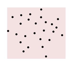
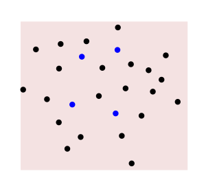
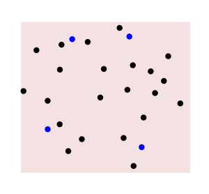
- Or: a
de-correlated, zero-mean
point cloud has a small subset that [after normalization] is
nearly de-correlated, nearly zero-mean
Spectral Sparsification
- `A` has the form `RQ`
- `Q` is `d\times n` and has orthonormal rows
- `R` is triangular
- (Gram-Schmidt on rows)
- Where `|\gamma| \le \epsilon`
- A good spectral approximation
What Can Be Estimated
if `D` is Known
- Eigenvalues of `AA^\top`
- Least-squares regression `\min\{\norm{A^\top x}^2 | x\in\reals^d, x_d=1\}`
- `-A_{d:}^\top` is RHS
- Probabilities `\rho(j)` are roughly the statistical leverage scores
- Spectral sparsifier `G'` of graph `G` with `d` nodes
- `G'` has `m` edges, Laplacian `L(G')` eigenvalues `\approx L(G)` eigenvalues
- `A` is a scaled version of `G`'s vertex-edge incidence matrix
- `m=O(d/\epsilon^2)` is possible [BSS09]
Finding the Weights?
- But: how to find `D`?
- Finding `RQ` factorization may be too much work
- Can be done in `\tilde{O}(\nnz{G})` for `L(G)`
- A random rotation makes `\rho(j)` uniform
- Helpful in regression case
`D` as Almost-a-Coreset for MEE
- Minimum Volume Enclosing Ellipsoid `\MEE(A)`
- Critical/Contact/Support/Basis Points: `A'\subset A` with
- `\MEE(A) = \MEE(A')`
- `|A'|\le d(d+1)/2`
- Suppose:
- `A` is centrally symmetric (`x\in A \iff -x\in A`), so MEE centered at origin
- `A=A'`; throw away non-critical points
`D` as Almost-a-Coreset for MEE, II
- Then there is linear `N : \reals^d \rightarrow \reals^d` with: [John]
- `N(\MEE(A)) = \Ball`
- Columns of `NA` are unit vectors
- There is a column scaling `\hat{D}` so that rows of `NA\hat{D}` are orthogonal
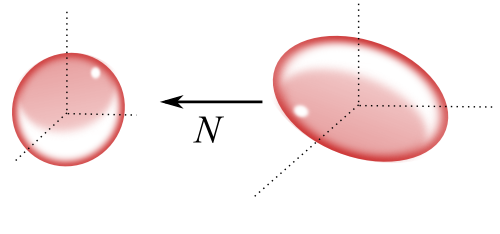
`D` as Almost-a-Coreset for MEE, III
- The `D` matrix for `NA\hat{D}` has `NA\hat{D}^2DA^\top N^\top = I+E`
- So `NA D^{1/2}` selects columns of `NA`, yields almost orthogonal matrix
- This implies: there is a perturbed version of `NAD^{1/2}` whose MEE is close to `\MEE(A)`
- That is, roughly: there are coresets for MEE of size `O((d\log d)/\epsilon^2)`
- (Not like Kumar/Yildirim coresets)
A Primal-Dual MEB Algorithm
- For other QP problems, need a primal-dual approach
- Restating weak duality: $$\max_{p\in\Delta} -(\norm{Ap}^2 + p^\top b) \le \min_{x\in\reals^d} \max_{p\in\Delta} \sum_{i\in[n]} p(i)\norm{x-A_i}^2 = R_{A}^2$$
Max `p` vs. Min `x`
For rounds `t=1,\ldots T`, two players respond to each other with `p_t` and `x_t`- The "min player" tries to find the minimizing `x_t`
- For given `p`, the best `x` is `Ap`, the weighted centroid of the input points
- Less myopically, `x_{t+1}\leftarrow \frac{1}{t}\sum_{\tau\in[t]} Ap_\tau`
- The "max player" tries to find the maximizing `p_t\in\Delta_n`
- For given `x`, a short-sighted response `p` has some `p(i)=1`
- Less short-sighted: `p_t(i) = p_{t-1}(i) \exp(\eta || x_{t-1} - A_i||^2)`
- For suitable value `\eta`
- ...and also normalizing so that `\sum_i p_t(i) = 1`
- That is, a Multiplicative Weights update
A Primal-Dual Algorithm
The resulting algorithm, in pseudo-code:
`p_1\leftarrow (\frac{1}{n}, \frac{1}{n}, \ldots, \frac{1}{n})`; `x_1 \leftarrow A p_1`;
for `t=1,\ldots,T-1`:
for each `i`: `p_{t+1}(i) \leftarrow p_t(i)\exp(\eta||x_{t} - A_i||^2)`
`p_{t+1}\leftarrow p_{t+1}/||p_{t+1}||_1`
`x_{t+1} \leftarrow (1-\frac{1}{t})x_t + \frac{1}{t}A p_{t}`
// So `x_{t+1} = A \sum_{\tau\in [t]} p_{\tau}/t`
return `\overline{x} \leftarrow \sum_{t\in[T]} x_t/T`;
The Primal-Dual Algorithm is Not Too Bad
- Claim: for `T=\tilde{O}(1/\epsilon^2)`, `\bar{x} = \sum_{\tau\in [T]} x_\tau/T` has $$R_A(\bar{x}) \le R_A(x^*) + \epsilon.$$
- Work per iteration is `O(\nnz{A})=O(nd)`
- Compute `Ap_t` and the squared distances `||x_t - A_i||^2` via `x_t^\top A
- Aside from finding `A p_t` and `A^\top x_t`, work is `O(n+d)`
Randomizing the Primal-Dual Algorithm
- We can use random estimates so that one iteration takes $O(n+d)$ total time
- To update $x_t$, use `\ell_1` sampling:
- Pick $i_t$ with prob. $p_t(i)$, and use $A_{i_t}$ instead of `A p_t`
- `\E[A_{i_t}] = A p_t`, so update is the same in expectation
- `x_{t+1}` is the centroid of `\{A_{i_\tau}\}_{\tau\in [t]}`, as in FW
- To update `p_t`, use `\ell_2` sampling for each `\norm{x_t - A_i}^2`
The Randomized Primal-Dual Algorithm is
Not Too Bad
- Claim: for `T=\tilde{O}(1/\epsilon^2)`, the output vector `\bar{x} = \sum_{\tau\in [T]} x_\tau/T` has $$R_A(\bar{x}) \le R_A(x^*) + \epsilon.$$
- NB: same as for deterministic version
- Time per iteration is `O(n+d)`
- Can be much faster than deterministic version
- But maybe there's big multipliers hiding in the `\tilde{O}()`?
Randomized vs. Deterministic
- Noise added to distances to simulate `\ell_2` sampling
- Color: large `\color{red}{p_t(i)}`, small `\color{blue}{p_t(i)}`,
HSL interpolation - Black dot is center `x_t` for randomized
- Black dot with red ring is center `x_t` for det.
- After some iterations, similar behavior
Related Work: Prior Primal-Dual Algorithms
- An analogous perceptron algorithm finds $$\min_{p\in\Delta_n} \max_{x\in\Ball_d} x^\top Ap $$
- Previous work [GK,KY] found sublinear approx. algorithms for $$\quad\quad\min_{p\in\Delta_n}\max_{x\in\color{green}{\Delta_d}} x^\top A p$$
- Optimal mixed strategies for a game
- Better results: small relative error
- Easier(?) problem, because `\ell_1` sampling is easier than `\ell_2` sampling
- `||A_i||_\infty \le ||A_i||_2`, or `\Delta_d\subset\Ball_d`
- (The solution to `\max_{p\in\Ball_n}\max_{x\in\Ball_d} x^\top A p` is `||A||`)
Concluding Remarks
- In ML, more training should give lower risk
- Touching 1000 sample points once may better than
touching 100 sample points 10 times each - Sample complexity may not be directly relevant
- Our [CHW] algorithms also good in this respect
- Touching 1000 sample points once may better than
- Geometric algorithms with runtimes akin to graph algorithms?
- Run-time as a function of number of nonzero entries ("number of edges")
- Or sparsity `=` max nonzeros per point = max degree
- Run-time as a function of number of nonzero entries ("number of edges")
- Are there `\tilde{O}(\nnz{A})` algorithms for these problems?
- NN search: improvements using `\ell_2` sampling
Thank you for your attention