Sketching Matrices

Slides for SLMath Summer School
The Mathematics of Big Data: Sketching and (Multi-) Linear Algebra
(Slides on matrix sketching)
Ken Clarkson
IBM Research

In the html version, navigate with arrow keys, or arrowset in lower right of slides;
major sections navigate "left and right", within sections "up and down"

Introduction, Algorithmic Motivation

\( \newcommand\norm[1]{|| #1 ||} \newcommand{\norme}[1]{{\myvertiii{#1}}} \newcommand{\myvertiii}[1]{{\left\vert\kern-0.2ex\left\vert\kern-0.2ex\left\vert #1 \right\vert\kern-0.2ex\right\vert\kern-0.2ex\right\vert}} \newcommand\E{\mathrm{E}} \DeclareMathOperator\Var{Var} \DeclareMathOperator\Cov{Cov} \DeclareMathOperator\stdev{Stdev} \DeclareMathOperator\cgf{CGF} \DeclareMathOperator\Prob{Pr} \DeclareMathOperator\subg{subG} \DeclareMathOperator\dist{dist} \DeclareMathOperator\KJL{K_{JL}} \newcommand\nnz[1]{{\textrm{nnz}(#1)}} \DeclareMathOperator\Dist{\mathbf{Dist}} \DeclareMathOperator\diam{diam} \DeclareMathOperator\reals{{\mathrm{I\!R}}} \DeclareMathOperator\R{{\mathrm{I\!R}}} \DeclareMathOperator\poly{poly} \DeclareMathOperator\polylog{polylog} \DeclareMathOperator\rank{rank} \DeclareMathOperator\im{im} \DeclareMathOperator\range{im} \DeclareMathOperator\rowspan{rowspan} \DeclareMathOperator\colbasis{colbasis} \DeclareMathOperator\trace{tr} \DeclareMathOperator\diag{diag} \DeclareMathOperator\argmin{argmin} \DeclareMathOperator\Err{{\mathtt{NE}}} \newcommand\eps{{\epsilon}} \DeclareMathOperator\argmax{argmax} \DeclareMathOperator\cost{cost} \DeclareMathOperator\OPT{{\mathtt{OPT}}} \DeclareMathOperator\sr{sr} \DeclareMathOperator\sd{{\mathtt{sd}}} \newcommand\cN{{\mathcal N}} \newcommand\cR{{\mathcal R}} \newcommand\cP{{\mathcal P}} \newcommand\cS{{\mathcal S}} \newcommand\cL{{\mathcal L}} \newcommand\cD{{\mathcal D}} \newcommand\cM{{\mathcal M}} \newcommand\cE{{\mathcal E}} \newcommand\cC{{\mathcal C}} \newcommand\tO{{\tilde O}} \newcommand\hphi{{\hat\phi}} \newcommand\symd[1]{#1^\top#1 - \Iden} \newcommand\twomat[2]{\left[\begin{smallmatrix} #1 \\ #2 \end{smallmatrix} \right] } \newcommand\maybemathbf[1]{\mathbf{#1}} \DeclareMathOperator\bfone{{\mathbf{1}}} \newcommand\mZero{\maybemathbf{0}} \newcommand\Iden{\maybemathbf{I}} \newcommand\mSig{\maybemathbf{\Sigma}} \newcommand\mLam{\maybemathbf{\Lambda}} \newcommand\mPi{\maybemathbf{\Pi}} \newcommand\mA{\maybemathbf{A}} \newcommand\mB{\maybemathbf{B}} \newcommand\mC{\maybemathbf{C}} \newcommand\mD{\maybemathbf{D}} \newcommand\mE{\maybemathbf{E}} \newcommand\mG{\maybemathbf{G}} \newcommand\mH{\maybemathbf{H}} \newcommand\mM{\maybemathbf{M}} \newcommand\mN{\maybemathbf{N}} \newcommand\mP{\maybemathbf{P}} \newcommand\mQ{\maybemathbf{Q}} \newcommand\mR{\maybemathbf{R}} \newcommand\mS{\maybemathbf{S}} \newcommand\mT{\maybemathbf{T}} \newcommand\mU{\maybemathbf{U}} \newcommand\mV{\maybemathbf{V}} \newcommand\mW{\maybemathbf{W}} \newcommand\mX{\maybemathbf{X}} \newcommand\mY{\maybemathbf{Y}} \newcommand\mZ{\maybemathbf{Z}} \newcommand\va{\maybemathbf{a}} \newcommand\vb{\maybemathbf{b}} \newcommand\vd{\maybemathbf{d}} \newcommand\ve{\maybemathbf{e}} \newcommand\vg{\maybemathbf{g}} \newcommand\vh{\maybemathbf{h}} \newcommand\vm{\maybemathbf{m}} \newcommand\vp{\maybemathbf{p}} \newcommand\vr{\maybemathbf{r}} \newcommand\vs{\maybemathbf{s}} \newcommand\vw{\maybemathbf{w}} \newcommand\vx{\maybemathbf{x}} \newcommand\vy{\maybemathbf{y}} \newcommand\vz{\maybemathbf{z}} \newcommand\vtau{\boldsymbol{\tau}} \newcommand\tmA{\tilde{\maybemathbf{A}}} \newcommand\tmW{\tilde{\maybemathbf{W}}} \newcommand\tmZ{\tilde{\maybemathbf{Z}}} \newcommand\tmY{\tilde{\maybemathbf{Y}}} \newcommand\tmX{\tilde{\maybemathbf{X}}} \newcommand\tmV{\tilde{\maybemathbf{V}}} \newcommand\tmH{\tilde{\maybemathbf{H}}} \newcommand\bmP{\bar {\maybemathbf{P}}} \newcommand\tvx{\tilde{\maybemathbf{x}}} \newcommand\tva{\tilde{\maybemathbf{a}}} \newcommand\tvb{\tilde{\maybemathbf{b}}} \newcommand\hmY{\maybemathbf{\hat Y}} \newcommand\hmS{\maybemathbf{\hat S}} \newcommand\hmR{\maybemathbf{\hat R}} \newcommand\hmA{\maybemathbf{\hat A}} \newcommand\hvb{\hat {\maybemathbf{b}}} \)

Outline

Randomized Estimation
Algorithms for
Linear Algebra

Outline

Linear Algebra
Randomized Estimation
Algorithms

Regression

`\mA,\vb,n,d,\mA_{i*}` `\mA` is an `n\times d` matrix
`\vb\in\R^n` is a column vector
`\mA_{i*}` is row `i` of `\mA`

`(\mA_{i*}, b_i)` for `i \in [n]` is an input set of points

(General) regression Given function `M:\R\rightarrow\R`,
find $$\min_{\vx\in\R^d} \sum_i M(\mA_{i*} \vx - b_i)$$ Generically, an `M`-estimator.
`\mA\vx - \vb` is the residual

`\ell_p` regression When:

`M(z)=z^2`, least-squares regression [G95][L05]
- Minimize the Euclidean norm `\norm{\mA\vx - \vb}` of the residual
`M(z)=|z|^p` for some `p\ge 1`, `\ell_p` regression
`\qquad` e.g., `p=1`, a.k.a. least absolute deviations

Least squares is still important

Besides immediate data science applications,
least squares can be in the "inner loop" for:

Interior point methods for linear programming
Multiple-response least-squares with manifold constraints
Generalized linear models
Training neural networks
Tensor decomposition

(Some) notation and conventions

In one place, in case I forget to say

Matrices, e.g. `\mA`, are denoted with bold upper case
`\mA_{i*}` is row `i` of matrix `\mA`
`\mA_{*j}` is column `j` of `\mA`
`a_{ij}` (or sometimes `A_{ij}`) are entries of matrix `\mA`
Vectors, e.g. `\vx`, are bold lower case, and are columns unless otherwise indicated
Entries of matrices and vectors are real numbers
`\nnz{\mA}` is the number of nonzero entries of `\mA`: often, the input size
`\norm{\vx}` is the Euclidean norm
`\norm{\mA}_2` is the spectral norm (sometimes, dropping the subscript 2)
`\mA^\top\in\R^{d\times n}` is the transpose, with entries `A^\top_{ji} = A_{ij}` for `i\in [n], j\in [d]`
`\mA^+\in\R^{d\times n}` is the Moore-Penrose pseudo-inverse, with `\mA\mA^+\mA = \mA`, `\mA^+\mA\mA^+=\mA^+`
`\Iden_d\in\R^{d\times d}` is the identity matrix, with entries `I_{ii}=1`, and 0 otherwise;,
`\ve_i\in\R^n`, for `i \in[n]` are the natural basis (standard basis) vectors
`\qquad` where `\ve_i = \Iden_{i*}`, with `i`'th coordinate 1, and 0 otherwise.
`\im(\mA)\equiv \{\mA\vx \mid \vx\in\R^d\}` is the image (a.k.a. column span, range) of `\mA\in\R^{n\times d}`
`\rank(\mA) \equiv \dim(\im(\mA))`
`\trace(\mA) = \sum_i a_{ii}`, the sum of the diagonal entries
`\diag(\vd)`, for `\vd\in\R^n`, is the diagonal matrix `\mD\in\R^{n\times n}` with `D_{ii}=d_i`

`[n]\equiv\{1,2,\ldots,n\}`, for positive integer `n`
`a\wedge b` denotes `\min\{a,b\}`, for `a,b\in\R`
`g(n)=O(f(n))` as `n\rightarrow\infty` denotes `\exists C,n_0` with `n\ge n_0\implies g(n)\le Cf(n)`; `\tO(f)` denotes `f\log^{O(1)}f`
`x=(1\pm \eps)y` means, for real `x,y` and `\eps\ge 0`, that `|x-y| \le \eps |y|`
`x\approx_\eps y` means `x=(1\pm\eps)y`
`\poly(k)` means `k^{O(1)}`

Low-rank approximation: fitting data

Given: points `\mA_{*j}` as columns of matrix `\mA`
Fit: a `k`-dimensional subspace `L_k^*` minimizing $$\cost(\mA,L) \equiv \sum_{j\in [d]} \dist(\mA_{*j},L)^2$$

`L=\im(\mY)=\{\mY\vx\mid\vx\in\R^k\}` for some `\mY\in\R^{n\times k}`
So `\mA_{*j}\approx\mY\vx`, for some `\vx\in\R^k`,
that is, a linear combination of the columns of `\mY`.

Making this column `\mX_{*j}` of matrix `\mX\in\R^{k\times d}`, and the distance Euclidean,
we are solving, for all `j\in[d]`, the least-squares problem
`\min_{\mX_{*j}\in\R^k} \norm{\mA_{*j}-\mY\mX_{*j}}^2`. Putting these together:

Given `\mA\in\R^{n\times d}`, find $$\qquad\qquad\quad\argmin_{\substack{\mY\in\R^{n\times k}\\ \mX\in\R^{k\times d}}} \norm{\mA - \mY\mX}_F^2,$$ where the Frobenius norm `\norm{\mE}_F^2 \equiv \sum_{ij} e_{ij}^2`

For fixed `\mY`, the problem is least-squares regression for each column of `\mA` and corresponding column of `\mX`

For fixed `\mX`, least-squares for each row of `\mA` and corresponding row of `\mY`

Randomized approximation

These problems involve norms of vectors and/or matrices:
- `\norm{\mA\vx-\vb}`, the norm of the least-squares residual
- `\norm{\mA-\mY\mX}_F`, the approximation error for `\mY\mX`
Squared norms are sums `\norm{\vw}^2=\sum_{i\in[n]} w_i^2`
To estimate sums, we can use randomization

Linearity of expectation, Markov's inequality, and union bounds

Any random variables `X,Y\in\R` and constants `\alpha,\beta\in\R` satisfy `\E[\alpha X + \beta Y] = \alpha\E[X] + \beta\E[Y]`.

So for random `\vx\in\R^d` and constant matrix `\mA\in\R^{n\times d}`, the `i`'th entry of `\E[\mA\vx]` is
`\E[\mA\vx]_i = \E[\mA_{i*}\vx] = \sum_{j\in[d]} a_{ij}\E[x_j] = \mA_{i*}\E[\vx]`; that is, `\E[\mA\vx]=\mA\E[\vx]`.

A nonnegative random variable `X` and satisfies `\Prob\{X\ge t\} \le \E[X]/t` for all `t\gt 0`.

Any collection of random events `E_i` satisfies `\Prob\{\cup_i E_i\} \le \sum_i \Prob\{E_i\}`.

Let `X_i=1` when `E_i` occurs, and 0 otherwise. Then

`\begin{align*} \Prob\{\cup_i E_i\} & = \Prob\{\textstyle\sum\nolimits_i X_i \gt 0\} \\ & \le \E[\textstyle\sum\nolimits_i X_i] \qquad \mathrm{\ Markov\ inequality}, t=1 \\ & = \textstyle\sum\nolimits_i \E[X_i] \qquad \mathrm{\ linearity\ of\ } \E \\ & = \textstyle\sum\nolimits_i \Prob\{E_i\} \end{align*}`.

Product and norm estimation using randomization

If a random distribution on `\vs\in\R^n` has
entries `s_i` with `\E[s_i^2]=1` for `i\in [n]` and `\E[s_is_j]=0` for `i,j\in [n], i\ne j`
then for `\vx,\vy\in\R^n`, `\E[(\vs\cdot\vx)(\vs\cdot\vy)] = \E[(\vs^\top \vx)(\vs^\top \vy)] = \E[\vx^\top\vs\vs^\top\vy] = \vx^\top\vy`.
In particular, `\E[(\vs^\top\vy)^2] = \E[\vy^\top\vs\vs^\top\vy] = \vy^\top\vy = \norm{\vy}^2`.

By hypothesis, `\E[\vs\vs^\top] = \E\left[ \begin{matrix} s_1^2 & s_1s_2& \ldots & s_1s_n \\ s_2s_1 & s_2^2 & \ldots \\... \\ s_ns_1 & s_ns_2 & \ldots & s_n^2 \end{matrix}\right] = \Iden_n = \left[ \begin{matrix} 1 & 0& \ldots & 0 \\ 0 & 1 & \ldots \\... \\ 0 & 0 & \ldots & 1 \end{matrix}\right].`

So `\E[\vx^\top\vs\vs^\top\vy] = \vx^\top\E[\vs\vs^\top]\vy = \vx^\top\Iden_n\vy= \vx^\top\vy.`

Sketching
`s_i \sim \cN(0,1)` independent

Since `\E[s_i]=0`, `\E[s_i^2] = \Var(s_i)=1`.
For `i\ne j`, independence implies `\E[s_is_j]=\E[s_i]\E[s_j]=0`.

Sampling
Pick `k\in[n]` with prob. `\frac1n`, `s_k\gets \sqrt{n}`, `0` o.w.

`\E[s_i^2] = \frac{1}{n}\sqrt{n}^2 + (1-\frac{1}{n})0 = 1`.
Also `s_i\ne 0 \implies s_j=0` for `i\ne j`,
`\quad` so `s_is_j=0`.

Speed: we can estimate `\norm{\mA\vx-\vb}^2\text{ by }(\vs^\top(\mA\vx - \vb))^2.`

Since `\vs^\top(\mA\vx - \vb) = (\vs^\top\mA)\vx - (\vs^ \top\vb),`
this is faster for multiple `\vx`,
(even for sketching)
if `\vs^\top\mA` and `\vs^\top\vb` are pre-computed.

Accuracy: not so good

Algorithms

With repetition and better distributions, randomization can be much more accurate.

Repetition means:

If a random distribution on `\mS\in\R^{m\times n}` has
independent rows, each row `\frac{1}{\sqrt{m}}` times an AMM vector,
then $$\E[\mS^\top \mS] = \E[\sum_{i\in[m]} [\mS_{i*}]^\top \mS_{i*}] = \sum_{i\in[m]} \E[[\mS_{i*}]^\top \mS_{i*}] = \sum_{i\in [m]} \frac{1}{m}\Iden = \Iden,$$ so for `\vx,\vy\in\R^n`, `\E[(\mS\vx)\cdot (\mS\vy)] = \E[\vx^\top\mS^\top \mS\vy] = \vx^\top\E[\mS^\top \mS]\vy = \vx^\top\vy`.
In particular, `\E[\norm{\mS\vy}^2] = \norm{\vy}^2`.

Many things can be done with such sketching matrices: there is a large cross-product $$\text{Randomized techniques} \times \text{Matrix problem} \times \left\{\begin{matrix} \text{Cost measures}\\ \text{Regularizations} \\ \text{Kernelizations} \end{matrix} \right\}$$ as will be described.

Next: basic results for least squares and sketching

`\eps`-approximations

`\eps`-approximation, `\tvx`, `\vx^*` For error parameter `\eps`, want a small relative-error solution:
`\tvx` such that $$\norm{\mA\tvx - \vb} \le (1+\epsilon) \norm{\mA\vx^* - \vb},$$ where `\vx^*\equiv \argmin_{\vx\in\reals^d} \norm{\mA\vx - \vb}`

The above will be the main focus here, but also of interest (maybe more interest) is minimizing `\norm{\tvx - \vx^*}`;
cf. section on pre-conditioned least squares.

Sketching Matrices:
Oblivious Subspace Embeddings

(Earlier, some distributions where `\E[\norm{\mS\vy]}^2] = \norm{\vy}^2`.)

Matrix `\mS\in\R^{m\times n}` is an `\eps`-embedding of set `\cP\subset\R^n` if $$\norm{\mS\vy }= (1\pm\eps)\norm{\vy }\text{ for all }\vy\in\cP.$$ `\mS` will be called a "sketching matrix".

`1\pm \eps` For real `x,y,\eps`, `x=(1\pm \eps)y` means that `|x-y| \le \eps|y|`

For `\mA\in\R^{n\times d}`,
a matrix `\mS ` is a subspace `\eps`-embedding for `\mA ` if `\mS ` is an `\eps`-embedding for `\im(\mA )= \{\mA\vx\mid\vx\in\R^d\}`. That is, $$\norm{\mS\mA\vx }= (1\pm\eps)\norm{\mA\vx }\text{ for all }\vx\in\R^d.$$ `\mS\mA` will be called a "sketch".

An oblivious subspace embedding is:

A probability distribution `\cal D` over matrices `\mS\in\R^{m\times n}`, so that
For any unknown but fixed matrix `\mA`,
`\mS ` is a subspace `\eps`-embedding for `\mA `, with high-enough probability.

Sketch and solve

Generic scheme using sketching:

				   generate sketching matrix `\mS\in\R^{m\times n}`,

				   compute `\mS\mA` and `\mS\vb`

				   return `\tvx := \argmin_{\vx\in\R^d} \norm{\mS(\mA\vx-\vb)}`

For least squares, the sketched problem is easy
But a similar approach applies to harder problems,
yielding greater speedup

Figure is not to scale: typically `m = \poly(d/\eps)`, of interest when `n\gg d`

Subspace embeddings for sketch and solve

Suppose `\mS` is a subspace `\eps`-embedding for `\im([\mA\ \vb])`.
Letting $$\begin{align*} \tvx\equiv & \argmin_{\vx\in\R^d}\norm{\mS (\mA\vx -\vb)} \\ \vx^*\equiv & \argmin_{\vx\in\R^d}\norm{\mA\vx -\vb} \end{align*}$$ when `\eps\le 1/3` $$ \norm{\mA\tvx-\vb} \le (1+3\eps)\norm{\mA\vx^*-\vb} $$

`\approx_\eps` For `a,b\in\R`, `\eps\ge 0`, let `a\approx_\eps b` mean that `|a-b|\le \eps|b|`, that is, `a=(1\pm\eps)b`.

For `\vy=\left[\begin{smallmatrix}\vx\\ -1\end{smallmatrix}\right]`, `\vx\in\R^d`, $$\norm{\mS (\mA\vx -\vb)} = \norm{\mS[\mA\ \vb]\vy} \approx_\eps\norm{[\mA\ \vb]\vy} = \norm{\mA\vx -\vb}$$ So
$$ \begin{align*} \norm{\mA\tvx-\vb} & \le\frac{\norm{\mS (\mA\tvx-\vb)}}{1-\eps} \le\frac{\norm{\mS (\mA\vx^*-\vb)}} {1-\eps} \le\norm{\mA\vx^*-\vb}\frac{1+\eps}{1-\eps}, \end{align*}$$
and so for `\eps\le 1/3`, `\norm{\mA\tvx-\vb}\le\norm{\mA\vx^*-\vb}(1+3\eps)`.

Solving least-squares in "sketch space"
yields a good solution in the original space.

Good sketching matrices

Criteria, for given `\eps`:

Speed of computation of `\mS`
Speed of computation of `\mS\mA`
Sketching dimension `m`,
where `\mS\in\R^{m\times n}`

time for `\mS\mA` is `O(ndm)`, `m=\tO(d/\eps^2)`:
`\quad` Johnson-Lindenstrauss (JL), i.i.d subGaussians
`\tO(nd)`, `m = \tO(d/\eps^2)`:
`\quad` Fast JL, Subsampled Randomized Hadamard
`\tO(\nnz{\mA})`, `\tO(d^2/\eps^2)`:
`\quad` Countsketch, a.k.a. sparse embeddings
`\quad` cf. "feature hashing", maybe "random indexing"
`\tO(\nnz{\mA}) +\tO(d^3)`, `\tO(d/\eps^2)`:
`\quad` Two-stage
`\tO(\nnz{\mA}f(\kappa))`, `\tO(d^{1+\kappa}/\eps^2)`:
`\quad` OSNAPs
`O(\nnz{\mA}\log(d)/\eps)`, `O(d\log(d)/\eps^2)`:
`\quad` Sparse embeddings
time to find `\mS` is `O(\nnz{\mA}\log(d)) + \tO(d^3)`, `m=O(d\log(d)/\eps^2)`
`\quad` Leverage-score sampling

The bottom line: quickly reduce `n` to `\poly(d)`
Actually even better: to `\poly(\rank(A))`,
that is, polynomial in the dimension of the `\im(\mA)`.

Algorithmic problems beyond regression

Sketching can be applied to a variety of NLA problems

Rank: `\tO(\nnz{\mA}) + \rank(\mA)^3` (cf. rank condensers)
- `\rank(\mA)\equiv \dim (\im(\mA))`
Trace
- `\trace(\mA) \equiv \sum_{i\in[n]} a_{ii}\quad`(only defined for square `\mA`, `n=d`)
Regression
- `\tO(nd) + \tO(d^3)\poly(1/\eps)`
- `\tO(\nnz{\mA}) + \tO(d^3)\poly(1/\eps)`
- `\tO(\nnz{\mA})\log(1/\eps) + \tO(d^3)\poly(\log(1/\eps))`
- `\tO(\nnz{\mA} + \tO(d^3)\poly(1/\eps))`
Low-rank approximation
- `\tO(\nnz{\mA}) + O(n+d)\poly(k/\eps) + \poly(k/\eps)`
Leading eigenvalues
- `\tO(\nnz{\mA}) + \poly(k/\eps)`
Canonical correlation analysis
- `\tO(\nnz{\mA}+\nnz{\mB}) + \tO(d^3)\poly(1/\eps)`
CUR decomposition
Dimensionality reduction for `k`-means

Excluding near-linear for constant `\eps`, fast matrix multiply, non-relative error
No dependence on condition number, incoherence, or other `\mA` numerical properties
May require large `\nnz{\mA}\gg d` and/or not-too-small `\eps` to be "near-linear"

A sample of other uses of sketching

Matrix-free computations: using only matrix-vector products
- E.g., rank-`k` approx., `\eps` relative error, `\tO(k\eps^{-1/3})` matrix-vector products
Hyperdimensional computing (Vector Symbolic Architectures)
- Sketching of characteristic vectors of sets
Low-rank Semidefinite Programming (SDP)
- For iterative optimizations where the output is low-rank matrix
  Approach: maintain sketch that is a good low-rank approximation to iterates
Online learning of general recurrent computational graphs such as recurrent network models.
- Independent invention of sketching
Quantum-inspired algorithms: comparable to quantum in an apples-to-apples comparison [T19] [CCHLW22] [BT23]

More `\tO(\nnz{\mA})`, not using sketching

Elementwise sampling plus iterative methods, for
- Low-rank approximation [BJS14]
- Robust PCA [NNSAJ14]
- Matrix completion [H13][JNS13][HW14]
Need numerical conditions on matrix (incoherence)
Matrix completion
- Cost on error `\mE` is not `\norm{\mE}_F^2` but `\norm{\mE}_\Omega \equiv \sum_{(i,j)\in\Omega} E_{ij}^2`
  - For `\Omega\subset [n]\times[d]`
  - Random `\Omega\implies` can `\approx` let missing entries be zero
- `\poly(\log(1/\eps))` instead of `\poly(1/\eps)`

Extension: kernelization

That is, linearizing non-linear problems

Map rows `\mA_{i*}` to `\phi(\mA_{i*})` in higher dimension
- For example, add values `a_{i1}a_{i2}` for each `i` to capture interation of two variables
  (That is, a new column comprising the entrywise product of `\mA_{*1}` and `\mA_{*2}`)
- Change geometry to discount large distances (Gaussian kernel)
Map `\phi(\mA_{i*})` to lower dimension, preserving `\phi(\mA_{i*})^\top\phi(\mA_{j*})`
1. And so, a kind of sketching

Extension: robustness

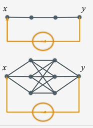
Least squares is not very robust, fits with other measures are better

Fitting to black dots together with green dot
Red line from least-squares

The green point can exercise a lot of leverage

Green line is for `\ell_1` regression `M(z)=|z|` above
`\tO(\nnz{\mA}) + \poly(d/\eps)` [C05][LMP13][CW13][CohP14]
- And much since

Extension: regularization

Given `\mA\in R^{n\times d}`, `\vb\in\R^n`, `\lambda \ge 0`.
Find $$ \min_{\vx \in \R^d} \norm{\mA\vx-\vb}^2 \color{green}{ + \lambda\norm{\vx}^2} $$

Regularization reduces large variations in `\vx`, lowers sample complexity

Course outline

"Some" "basics"
Oblivious sketching matrices with independent entries
- Approximate Matrix Multiplication (AMM)
AMM and Embedding
Countsketch
- Least-squares and AMM
Pre-Conditioned Least Squares
Sampling: length-squared and leverage-score
Subsampled Randomized Hadamard Transform
Multiple-response least-squares regression, low-rank approximation
Oblivious sketches: Sub-Gaussian Matrices
Trace Estimation (Shashanka)
Subspace iteration, Krylov methods (Shashanka)
(Maybe) Random Fourier features

Next week:

Tensor CP Foundations (Tammy)
Tensor CP randomized algorithms (Tammy)
Tucker decomposition (Misha + Lior)
T-product (TSVD) decomposition (Misha + Lior)

Some basics

Orthonormal matrices, projection

`\mU\in\R^{n\times d}` is orthonormal if `\mU^\top\mU = \Iden`, that is,
its columns are unit vectors, and are pairwise orthogonal. (This terminology is not used by everyone.)

If `\mU` is orthonormal and square, it is orthogonal, and `\mU\mU^\top=\Iden`

A symmetric matrix `\mP` of the form `\mP_\mU=\mU\mU^\top` (or just `\mP`) is an orthogonal projection matrix, and `\mP\mP=\mP` .
(We'll just say "projection", but, not all projections are orthogonal.)

If `\mU` has orthonormal columns, so `\mU^\top\mU=\Iden`,
then `\norm{\mU\vy} = \norm{\vy}`.

`\norm{\mU\vy}^2 = \vy^\top\mU^\top \mU\vy = \vy^\top\Iden\vy = \norm{\vy}^2`.

If `\mP` is a (orthogonal) projection matrix, then:
`\quad\bmP\equiv \Iden-\mP` is also a projection
`\quad\mP\bmP = 0 = \bmP\mP`
`\quad\norm{\vx}^2 = \norm{\mP\vx}^2 + \norm{\bmP\vx}^2\quad` (a.k.a. the Pythagorean theorem)
`\quad\norm{\mP}_F^2=\sum_{i,j} p_{ij}^2 = \rank(\mP)`.

The closest vector to `\vy` in `\im(\mU)` is `\mU\mU^\top\vy=\mP_\mU\vy`.

Left as an exercise.

Let `\mP` denote `\mP_\mU`. Then `\mP\vy\in\im(\mU)`, and if `\vz\in\im(\mU)`, then `\mP\vz = (\mU\mU^\top)\mU\vz' = \vz` and `\bmP\vz = \bmP\mP\vz=0`, implying
`\begin{align*} \norm{\vy-\vz}^2 & = \norm{\bmP(\vy-\vz)}^2 + \norm{\mP(\vy-\vz)}^2 \\ & = \norm{\bmP\vy}^2 + \norm{\mP\vy - \vz}^2 \\ & \ge \norm{\bmP\vy}^2 = \norm{\vy - \mP\vy}^2, \end{align*}`
the squared distance of `\vy` to `\mP\vy`.

The singular value decomposition

For every matrix `\mA\in\R^{n\times d}`, there are matrices
`\mU\in\R^{n\times n}`, `\mSig\in\R^{n\times d}`, and `\mV\in\R^{d\times d}`
such that $$\mA = \mU\mSig\mV^\top,$$ where

`\mU^\top \mU = \Iden_n\quad` (`\mU` is an orthogonal matrix)
`\mV^\top \mV = \Iden_d\quad` (`\mV` is an orthogonal matrix)
`\mSig` is a diagonal matrix (`\sigma_{ij}=0` if `i\ne j`),
and has nonnegative entries `\mSig_{ii} = \sigma_i(\mA) \ge 0` on the diagonal, for `i\in[n\wedge d]` with `\sigma_i` nondecreasing in `i`

`\rank(\mA)=\dim(\im(\mA))` is the number of nonzero entries of `\mSig`

`\mA=\mU\mSig\mV^\top` can be written `\mA = \sum_i \sigma_i(\mA)\mU_{*i}\mV_{*i}^\top`.
`\quad`(Here `\mV_{*i}^\top=[\mV_{*i}]^\top`, the transpose of the `i`'th column of `\mV`.)

If there are `r = \rank(A) \lt n\wedge d` nonzero singular values,
often the SVD is written as $$\mA = \mU\mSig\mV^\top,$$ where `\mU\in\R^{n\times r}`, `\mSig\in\R^{r\times r}`, and `\mV\in\R^{d\times r}`,
with the parts that contribute zero omitted. Here `\mSig` is invertible.

Best rank-`k` approximation The solution to the low-rank approximation problem $$A_k = \argmin_{\mX:\rank(\mX)=k}\norm{\mX-\mA}_F$$ is `\mA_k = \sum_{i\in[k]} \sigma_i(\mA)\mU_{*i}\mV_{*i}^\top`, that is, `\mU_{*,1:k}\mSig_k\mV_{*, 1:k}^\top`. `\mA_k` also is the closest in spectral norm `\norm{\cdot}_2`.

Eigendecomposition

For every square symmetric matrix `\mW\in\R^{n\times n}`,
there are matrices
`\mU\in\R^{n\times n}` and `\mLam\in\R^{n\times n}`
such that $$\mW = \mU\mLam\mU^\top,$$ where

`\mU^\top \mU = \Iden_n\quad` (`\mU` is an orthogonal matrix)
`\mLam` is diagonal, and has entries `\lambda_{ii} = \lambda_i(\mA)` on the diagonal, for `i\in[n]` with `\lambda_i` nondecreasing in `i`

For matrix `\mW`, if `\vy` and `\lambda` satisfy `\mW\vy = \lambda\vy`,
say that `\vy` and `\lambda` are an eigenvector and eigenvalue pair for `\mW`.

(Recall `\ve_i` has `e_i=1,e_j=0, j\ne i`)
For `\mW` with eigendecomposition `\mW=\mU\mLam\mU^\top`,
`\mW\mU_{*i} = \mU\mLam\mU^\top\mU_{*i} = \mU\mLam\ve_i = \mU \lambda_{ii}\ve_i = \mU_{*i}\lambda_{ii}`,
so `\mU_{*i}` and `\lambda_{ii} = \lambda_i(\mA)` are an eigenvector/eigenvalue pair.

The normal equations, the Moore-Penrose pseudo-inverse

Let `\vx^* \equiv \argmin_\vx\norm{\mA\vx - \vb}`. Then `\mA^\top\mA\vx^* = \mA^\top\vb`.

That is, `\vz^\top\mA^\top(\mA\vx^*-\vb)=0` for any `\vz`, so the residual `\mA\vx^*-\vb \perp\im(\mA)`

We use that `\vx^*` is also a minimizer of $$\norm{\mA\vx - \vb}^2 = (\mA\vx-\vb)^\top(\mA\vx - \vb) = \vb^\top\vb + \vx^\top\mA^\top\mA\vx - 2\vx^\top \mA^\top\vb,$$ which has the gradient `2\mA^\top\mA\vx - 2\mA^\top\vb`. The result follows by setting the gradient to zero.

Moore-Penrose pseudo-inverse `\mA^+` `\mA^+\equiv\mV\mSig^+\mU^\top`, for `\mA` with (any) SVD `\mA=\mU\mSig\mV^\top`,
where `\mSig^+` has nonzero entry `\sigma_i(\mA)^{-1}` in place of `\sigma_i(\mA)`

`\mA^+` properties `\mA^+=\mA^{-1}` when `\mA` is invertible
`\mA\mA^+\mA = \mA`
`\mA^+\mA\mA^+=\mA^+`
`\mA^+\mA = \Iden` when `\rank(\mA)= d` (`\mA` has full column rank)
`\mA^+ = (\mA^\top\mA)^+\mA^\top`, consistent with the normal eq.
`\mA^+\vb = \argmin_\vx\norm{\mA\vx - \vb}` (Also: mininum norm solution when there are many solutions)
`\mA^\top\mA\mA^+ = \mA^\top` (so `\mA^\top\mA\mA^+\vb = \mA^\top \vb`, consistent with the normal equations for `\mA^+\vb`)
`\mA\mA^+ = \mU\mU^\top=\mP_\mU` for `\mA=\mU\mSig\mV^\top` (thin), projection onto `\im(\mU)=\im(\mA)`.
`\mA^+\mA = \mV\mV^\top = \mP_\mV`, projection onto `\im(\mV)=\im(\mA^\top)`, the rowspace of `\mA`
`\mP_\mV = \mA^\top\mA^{+\top}`, so `\mA^\top\mA^{+\top}\mA^+\mA=\mA^+\mA`.
`\quad` (Where `\mA^{+\top} = (\mA^+)^\top`. This will matter, eventually.)

The `QR` decomposition

`QR` decomposition For `\mA\in\R^{n\times d}` with `n\ge d`, `\rank(\mA)=d`
there is `\mQ\in\R^{n\times d}` and `\mR\in\R^{d\times d}` where

`\mA = \mQ\mR`
`\mQ` has orthonormal columns, so `\mQ^\top\mQ = \Iden_d`
`\mR` is upper triangular, so `r_{ij}=0` for `i\gt j`

That is, `\im(\mQ)=\im(\mA)`, the columns of `\mQ` are an orthonormal basis for `\im(\mA)`.

`\mQ` and `\mR` can be computed in `O(nd^2)` time (via e.g. Gram-Schmidt orthogonalization).

The decomposition can be used for least squares:
`\mR^{-1}\mQ^\top\vb = \argmin_\vx\norm{\mA\vx - \vb}`, and:
`\quad`computing `\mQ^\top\vb` takes `O(nd)` time
`\quad`multiplying by `\mR^{-1}`, or really, solving `\mR\vx = \mQ^\top\vb`, takes `O(d^2)` time.

Pivoting (to deal with, for example, not-full-rank `\mA`) is ignored here, and the possibility that `\mR` is not invertible.

The spectral norm and eigenvalues

If `\vy_*\equiv \argmax_{\norm{\vy}=1} \norm{\mA\vy}`,
then there is `\lambda` so that `\mA^\top\mA\vy_* = \lambda\vy_*`, that is, `\vy_*` and `\lambda` are an eigenvector and eigenvalue pair for `\mA^\top\mA`.

(Loosely) We can use a Lagrange multiplier to obtain
$$\vy_* = \argmax_{\vy} \min_\mu \norm{\mA\vy}^2 + \mu*(\norm{\vy}^2 -1),$$ and setting the gradient with respect to `\vy` to zero, $$2\mA^\top\mA\vy = 2\mu\vy,$$ so `\vy_*` must satisfy this condition, with `\lambda=\mu`.

It follows that for `\lambda` the largest eigenvalue of `\mA^\top\mA`, and `\vy_*` the corresponding eigenvector, `\max_{\norm{\vy}=1} \norm{\mA\vy}^2 = \vy_*^\top\mA^\top\mA\vy_* = \vy_*^\top(\lambda\vy_*)=\lambda\vy_*^\top\vy_* = \lambda.`
It turns out that `\max_{\norm{\vy}=1} \norm{\mA\vy}^2 = \sigma_1(\mA)^2`, so `\sigma_1(\mA)^2 = \lambda_1(\mA^\top\mA)`.

The trace

The trace of square matrix `\mA\in\R^{n\times n}` is `\trace(\mA)=\sum_{i\in[n]} a_{ii}`.

Matrices assumed conformable to multiplication/addition,
meaning they have the right number of rows/columns to multiply/add.

`\trace(\mA\mB) = \trace(\mB\mA)`
`\qquad` So `\trace(\mA\mB\mC\mD) = \trace(\mD\mA\mB\mC)\qquad` (but `\bcancel{\trace(\mA\mB\mC\mD) = \trace(\mA\mC\mB\mD)}`)
`\trace(\mA+\mB) = \trace(\mA) + \trace(\mB)` (when conformable for addition)
`\E[\trace(\mX)] = \trace(\E[\mX])`
`\trace(\mA^\top) = \trace(\mA)`
`\trace(\mA^\top\mA) = \norm{\mA}_F^2 = \sum_{i,j} a_{ij}^2` (`\mA` need not be square)
`\trace(\mB\mA\mB^{-1}) = \trace(\mB^{-1}\mB\mA)= \trace(\mA)`, for invertible `\mB`
`\trace(\mA) = \trace(\mLam)` for eigendecomposition `\mA = \mU\mLam\mU^\top`

Suppose random `\vs\in\R^n` has `\E[\vs\vs^\top]=\Iden`.
Then `\E[\vs^\top\mA\vs]=\trace(\mA)`.

Via writing out the sum for `\vs^\top\mA\vs` and linearity of expectation , or,
`\trace(\mA) = \trace(\mA\E[\vs\vs^\top]) = \trace(\E[\mA\vs\vs^\top]) = \E[\trace(\mA\vs\vs^\top)] = \E[\trace(\vs^\top \mA \vs)] = \E[\vs^\top \mA \vs]`

Norms !

Suppose we have a vector space over the reals, and `\norm{\vx}` is a real-valued function.

For vectors `\vx,\vy`, `\qquad \norm{\vx+\vy}\le \norm{\vx} + \norm{\vy}`

For vectors `\vx` and scalars `\alpha\in\R`, `\qquad \norm{\alpha \vx} = |\alpha|*\norm{\vx}`

If `\norm{\cdot}` is subadditive and homogeneous, it is a seminorm. (And is nonnegative.)

For vectors `\vx`, if `\norm{\vx}= 0` only when `\vx=0`, then `\norm{\cdot}` is positive definite.
A seminorm with this property is a norm.

Hereafter, we use this notation for vectors and matrices

For `\vx\in\R^d`, we let `\norm{\vx}_p` denote `[\sum_i |x_i|^p]^{1/p}`,
and write`\norm{\vx}` for the Euclidean norm `\norm{\vx}_2`.

Given matrix `\mA`, `\norm{\vx}_\mA \equiv \norm{\mA\vx}` is a seminorm.

`\mS` is an `\eps`-embedding of `\im{\mA}` iff `\norm{\vx}_{\mS\mA} = (1\pm\eps)\norm{\vx}_{\mA}`.

Some norms: matrices

Let `\cS^{d-1}_p\equiv \{x\in\R^d \mid \norm{x}_p=1\}.`
(With `p` omitted when `p=2`, `d` omitted when in context).

For matrix `\mA`, let `\norm{\mA}_F^2\equiv \sum_{ij} a_{ij}^2`.

For matrix `\mA` and `p \ge 1`, let $$\norm{\mA}_p \equiv \sup_{\vx\in\cS_p} \norm{\mA\vx}_p.$$(With `p` omitted for `p=2`: the spectral norm.)

For symmetric matrix `\mW\in\R^{d\times d}` and non-empty `\cN\subset\R^d`, let $$\norm{\mW}_\cN \equiv \sup\{|\vx^\top\mW\vx|/\norm{\vx}^2 \mid \vx\in\cN, \vx\ne 0\},$$ so when `\cN\subset\cS`, `\norm{\mW}_\cN \equiv \sup_{\vx\in\cN} |\vx^\top\mW\vx|`.

Say that seminorm `\norm{\cdot}` is submultiplicative if it satisfies $$\norm{\mA\mB} \le \norm{\mA}*\norm{\mB}$$ for all (conformable) matrices `\mA` and `\mB`.

The Frobenius and induced norms satisfy submultiplicativity.
`\norm{\mA}_F = \sqrt{\sum_i \sigma_i(\mA)^2}`
`\norm{\mA}_2 = \sigma_1(\mA)`
`\norm{\mA\mB}_\xi \le \norm{\mA}_2*\norm{\mB}_\xi`, for `\xi \in \{F,\cN, 2\}`

Some norms: random variables

For real random variable `X` and `p\ge 1`, let `\norme{X}_p\equiv\E[|X|^p]^{1/p}`.

(Using `\norme{\cdot}` to distinguish moment norms from matrix/vector.)

If random variable `X\in\R` has `\E[X]=0`, say that `X` is centered.

For centered `X`, `\norme{X}_2^2 = \E[X^2] = \Var[X]`, so `\norme{X}_2 = \sd[X]`.

For real random variables `X` and `Y` and `p\ge 1`,
` \norme{X+Y}_p \le \norme{X}_p + \norme{Y}_p` (Minkowski),
and for `\alpha\in\R`, `\norme{\alpha X}_p = |\alpha|*\norme{X}_p`.

For `t\gt 0` and centered `X`, `\Prob\{|X|\ge t\} = \Prob\{|X|^p\ge t^p\}\le\norme{X}_p^p/t^p`.

For `p=1`, this is (more or less) Markov's inequality, and for `p=2`, Chebyshev.

For independent real random variables `X` and `Y`, `\Var[X+Y] = \Var[X] +\Var[Y]`.
That is, if also `\E[X]=\E[Y]=0`, then `\norme{X+Y}_2 = \sqrt{\norme{X}_2^2 + \norme{Y}_2^2}`, which is `\le \norme{X}_2 + \norme{Y}_2`.

We'll get to these eventually:

For real random variable `X`, `\norme{X}_{\psi_2} \equiv \sup_{p\ge 1}\norme{X}_p/\sqrt{p}.`
If `\norme{X}_{\psi_2}` is bounded, `X` is sub-Gaussian.

Matrix norms from sets: relation to spectral norms and embedding

For symmetric matrix `\mW\in\R^{d\times d}` and non-empty `\cN\subset\R^d`
let `\norm{\mW}_\cN \equiv \sup\{|\vx^\top\mW\vx|/\norm{\vx}^2 \mid \vx\in\cN, \vx\ne 0\}`
so when `\cN\subset\cS`, `\norm{\mW}_\cN \equiv \sup_{\vx\in\cN} |\vx^\top\mW\vx|`.

For `\mB\in\R^{m\times d}` and `\vx\in\R^d`, `\norm{\mB^\top\mB-\Iden}_{\{\vx\}} = |\vx^\top \mB^\top \mB\vx - \vx^\top\vx|/\norm{\vx}^2 = |\frac{\norm{\mB\vx}^2}{\norm{\vx}^2} - 1|`,
the distortion (error) of `\norm{\mB\vx}^2` in estimating `\norm{\vx}^2`.

For (sketching) matrix `\mB`, call `\mB^\top\mB-\Iden` the centered Grammian of `\mB`.

`\norm{\cdot}_\cN` and embedding of `\cN` For `\cN\subset\R^d` and `\mB\in\R^{m\times d}`, and `\beta\in (0,1]`,
`\norm{\symd{\mB}}_\cN \le\beta \implies \mB` is a `\beta`-embedding of `\cN\implies \norm{\symd{\mB}}_\cN \le 3\beta `.
If `\norm{\symd{\mB}}_\cS \le\beta` then `\mB` is a `\beta`-embedding of `\R^d`.

`\norm{\symd{\mB}}_\cN\le\beta` implies that `|\vx^\top(\symd{\mB})\vx| \le \beta\norm{\vx}^2,` for all `\vx\in\cN`,
that is, `\norm{\mB\vx}^2 = (1\pm\beta)\norm{\vx}^2`, so `\norm{\mB\vx} = (1\pm\beta)\norm{\vx}`.
The other implication follows using `(1+\beta)^2 \le 1+3\beta` and `(1-\beta)^2 \ge 1-3\beta`.
The last claim uses homogeneity of `\norm{\cdot}`.

`\norm{\cdot}` and embedding of `\cS` For symmetric `\mW`, `\norm{\mW }_2 = \sup_{\vy\in\cS} |\vy^\top\mW\vy| = \norm{\mW}_\cS.`

From the eigendecomposition `\mW=\mU\mLam\mU^\top` with `\mU` orthogonal and `\mLam` diagonal,
`\norm{\mW}_2^2 = \sup_{\vy\in\cS} \norm{\mW\vy}^2 = \sup_{\vy\in\cS} \norm{\mU\mLam\mU^\top\vy}^2 = \sup_{\vx\in\cS} \norm{\mLam\vx}^2 = \sup_{\vx\in\cS} \sum_i \lambda_{ii}^2 x_i^2 = \sup_i \lambda_{ii}^2`.
So `\norm{\mW}_2 = \sup_i |\lambda_{ii}|`.

Also `\norm{\mW}_\cS = \sup_{\vy\in\cS} |\vy^\top\mW\vy| = \sup_{\vy\in\cS} |\vy^\top\mU\mLam\mU^\top\vy| = \sup_{\vx\in\cS} |\vx^\top\mLam\vx| = \sup_{\vx\in\cS } |\sum_i \lambda_{ii}x_i^2|`,
so `\norm{\mW}_\cS = \sup_i |\lambda_{ii}|` as well.

From `\norm{\mW}_\cN` to `\norm{\mW}_2`: `\eps`-nets

`\cN= \cN(\epsilon)` is an `\epsilon`-net of set `\cal P` if it is both an:

`\epsilon`-packing: all `p\in\cN` at least `\epsilon` from `\cN`
- `D(p,\cN\setminus\{p\})\ge\epsilon` for `p\in\cN`
`\epsilon`-covering: all `p\in\cal P` at most `\epsilon` from `\cN`
- `D(p,\cN)\le\epsilon` for `p\in\cal P`, so `D(\cN,{\cal S})\le\epsilon`

We only really need the covering property, but a maximal packing is a minimal covering

Sphere covering number (NPH) The unit sphere in `\R^d` has an `\eps`-net of size at most `(1+\frac2\eps)^d`

(source)

`\norm{\mW}_{\cN_\eps}\approx\norm{\mW}_\cS = \norm{\mW}_2`

`\eps`-net bound For `\cN_{\eps}` an `\eps`-net of the unit sphere `\cS` in `\R^d` and `\eps\lt 1`,
if matrix `\mW ` is symmetric, then $$(1-2\eps)\norm{\mW }_2\le\norm{\mW }_{\cN_{\eps}}\le \norm{\mW}_\cS = \norm{\mW }_2.$$ and so if `\mB` is a `\beta`-embedding of `\cN_{\eps}`, where `\beta:= \norm{\symd{\mB}}_{\cN_\eps}`,
then it is a `\beta/(1-2\eps)`-embedding of `\cS`, and so of `\R^d`.

Since `\norm{\mW}_\cS=\norm{\mW}_2`, there is unit `\vy ` with `| \vy^\top\mW\vy | = \norm{\mW }_2`.

Since `\cN_\eps` is an `\eps`-net, there is `\vz` with `\norm{\vz}\le\eps` and `\vy -\vz\in\cN_{\eps}`.

We have
`\begin{align*} \norm{\mW }_2 & = | \vy^\top\mW\vy | = | (\vy -\vz)^\top\mW (\vy -\vz) +\vz^\top\mW\vy +\vz^\top\mW (\vy -\vz) | \\ & \le | (\vy -\vz)^\top\mW (\vy -\vz)| + |\vz^\top\mW\vy| + |\vz^\top\mW (\vy -\vz) | \\ & \le \norm{\mW }_{\cN_{\eps}} + \norm{\vz}*\norm{\mW\vy} + \norm{\vz}*\norm{\mW (\vy -\vz)} \\ & \le\norm{\mW }_{\cN_{\eps}} + 2\eps\norm{\mW }_2.\qquad\qquad (\norm{\vy}=\norm{\vy-\vz}=1) \end{align*}`

So `(1-2\eps)\norm{\mW }_2 \le\norm{\mW }_{\cN_{\eps}}`, as claimed.

Oblivious sketching matrices
with independent entries

The advantages of obliviousness

A random sketching matrix `\mS ` is oblivious if its distribution `\cal D`
does not depend on the input data.

Algorithmic advantages:

Construct `\mS ` without knowing input `\mA `
Streaming: when an entry of `\mA ` changes, `\mS\mA ` is easy to update
Distributed: if each processor `p` has matrix `\mA^{(p)}` and `\mA = \sum_p\mA^{(p)}`:
- Compute `\mS\mA^{(p)}` at each processor
- Ship to master for summation

Analysis advantages:

If `\mU` has `\im(\mU)=\im(\mA)`, then
condition `\cE` holds for `\im(\mA)` iff it holds for `\im(\mU)`.
So for analysis of oblivious sketching, WLOG `\mA` can be assumed orthonormal.

Independent Gaussian sketching matrices: embedding one vector

Recall the sufficient conditions for norm estimation vectors.

Given `\vy\in\R^n`.
If `\vg\in\R^n` has entries that are independent `\cN(0,1)`,
then `\vg^\top\vy\sim\cN(0,\norm{\vy}^2)`

The mean and variance follow from the norm estimation result above.
Also, a sum of independent Gaussians is Gaussian, and a scalar multiple of a Gaussian is Gaussian.

Given unit vector `\vy\in\R^n`, `\eps\in (0,1]`.
If `\mG\in\R^{m\times n}` has independent entries `g_{ij}\sim\cN(0, 1/m)`, then
$$\Prob\{|\,\norm{\mG\vy}^2 - 1| \ge \eps\} \le 2\exp(-\eps^2m/16).$$

That is, with high prob., `\mG` `\eps`-embeds unit `\vy\in\R^n`, and so any fixed `\vy\in\R^n`.

From just above, each entry of `\sqrt{m}\mG\vy` is `\cN(0,1)`, so its squared norm has a `\chi^2_m` distribution.
The standard bounds for the concentration of a `\chi^2_m` random variable `X` about its mean `m` imply $$\Prob\{|X-m|\ge 2\sqrt{m\alpha} + 2\alpha\} \le 2\exp(-\alpha).$$ Scaling by `1/m`, and letting `\alpha=\eps^2m/16`,
so that `2\sqrt{\alpha/m} + 2\alpha/m\le\eps`, the claim follows.

I.I.D. sketching matrices: embedding `\im(\mA)`

Given `\eps,\delta>0`, `\mA\in\R^{n\times d}`, unit vector `\vy\in\R^n`.
There is `m=O(\eps^{-2}d\log(1/\delta))` so that
If `\mS\in\R^{m\times n}` is randomly chosen from a fixed (oblivious to `\mA`) distribution with the property that
`\quad\mS` is an `\eps/6`-embedding of `\vy` with failure prob. at most `\delta'\equiv K_1\exp(-K_2\eps^2m)`, for some `K_1,K_2 \gt 0`,
then
`\quad\mS` is an `\eps`-embedding of `\im(\mA)` with failure prob. at most `\delta`.

Since `\mS` is oblivious, assume WLOG that `\mA` has orthonormal columns;
for some `\eps_0 > 0` to be determined, pick an `\eps_0`-net `\cN=\cN_{\eps_0}\subset\cS`;
for each `\vx\in\cN_{\eps_0}`, `\vy=\mA\vx\in\im(\mA)` is a unit vector (using `\mA^\top\mA=\Iden` and `\norm{\vx}=1`)
Let `\mW := \mA^\top\mS^\top \mS \mA - \Iden_d`,
so that `|\,\norm{\mS\vy}^2 - 1| = |\vy^\top\mS^\top\mS\vy - \vy^\top\vy| = |\vx^\top\mA^\top\mS^\top\mS\mA\vx - \vx^\top\mA^\top\mA\vx| = |\vx^\top\mW\vx|,` and thus
`\quad\norm{\mW}_{\{x\}}\le \eps/2` with failure prob. `\le\delta'`, from the hypothesis.
Applying this to all vectors in `\cN_{\eps_0}` and a union bound,
`\quad\norm{\mW}_{\cN_{\eps_0}} \le\eps/2` with failure prob. `\le\delta'|\cN_{\eps_0}|`.
Using the relation between `\norm{\mW}_\cS` and `\norm{\mW}_{\cN_{\eps_0}}` and the bound for `|\cN_{\eps_0}|`,
`\quad\norm{\mW}_\cS\le (\eps/2)/(1-\eps_0)` with failure prob. `\le\delta'|\cN_{\eps_0}|\le (1+\frac{2}{\eps_0})^d K_1\exp(-K_2\eps^2m)`
For fixed `\eps_0`, there is `m=O(\eps^{-2}d\log(1/\delta))` so that the failure probability is at most `\delta`.
For `\eps_0\le 1/2`, this implies`\norm{\mW}_\cS\le 2(\eps/2)=\eps`, and so the claim of the theorem.

Given `\delta,\eps>0`, and `\mA\in\R^{n\times d}`.
If `\mG\in\R^{m\times n}` has independent entries `g_{ij}\sim\cN(0, 1/m)`
then there is `m=O(\eps^{-2}d\log(1/\delta))` so that with failure probability at most `\delta`,
`\mG` is an `\eps`-embedding of `\im(\mA)`.

Given `\delta,\eps>0`, and `\mA\in\R^{n\times d}`.
If `\mS\in\R^{m\times n}` has independent entries `s_{ij}= \pm 1/\sqrt{m}`,
then there is `m=O(\eps^{-2}d\log(1/\delta))` so that with failure probability at most `\delta`,
`\mS` is an `\eps`-embedding of `\im(\mA)`.

Given `\delta,\eps>0`, and `\mA\in\R^{n\times d}`.
If `\mS\in\R^{m\times n}` has independent entries `s_{ij}\sim` sub-Gaussian, with `\E[\mS^\top\mS]=\Iden`,
then there is `m=O(\eps^{-2}d\log(1/\delta))` so that with failure probability at most `\delta`,
`\mS` is an `\eps`-embedding of `\im(\mA)`.

Aside 1/3: Gaussian Width and Gordon's theorem

Given `\cR\subset\R^n`, the Gaussian width of `\cR` is $$w(\cR)\equiv \E_{\vg\sim\cN(0,\Iden_n)} [\sup_{\vy,\vx\in\cR}\vg^\top(\vy-\vx)].$$

Note that `\sup_{\vg\in\cS}[\ldots]` is the (geometric) width, and `\E_{\vg\sim\mathrm{Unif}(\cS)}[\ldots]` is the mean width.

There are many variant definitions of Gaussian width, we will use the following.

Given `\cR\subset\R^n`, the Gaussian width of `\cR` is $$w(\cR)\equiv \E_{\vg\sim\cN(0,\Iden_n)} [\sup_{\substack{\vy\in\cR\\ \vy\ne 0}}\vg^\top\vy/\norm{\vy}].$$

(See also Rademacher complexity, using `\E_{\vg\sim\mathrm{Unif}(\{\pm 1\}^d)}[|\ldots|]`, and Gaussian complexity.)

`w(\R^n)\le\sqrt{n}` `\qquad`
`w(\cL)\le\sqrt{k}` for `\cL` a `k`-dimensional subspace `\qquad` (Hint: rotation invariance)
`w(\cR)\le\sqrt{2\log|\cR|}` for finite `\cR` `\qquad` (Hint: bound `\E[\exp(t*w(\cR))]`.)

Note that for finite `\cR`, its width can be much smaller than the given bound

Aside 2/3: Gordon's theorem and Johnson-Lindenstrauss

Gordon's theorem [G88] [MT21] For given `\cR\subset\R^n`,
if `\mG\in\R^{m\times n}` has independent entries `g_{ij}\sim\cN(0, 1/m)`, then $$\Prob\{\norm{\mG^\top\mG-\Iden}_\cR \ge 2\beta+\beta^2 \} \le \exp(-t^2/2),\text{ where } \beta\equiv \frac{w(\cR)+1+t}{\sqrt{m}}.$$

For a finite set `\cP\subset\R^n`, there is `m=O(\eps^{-2}(\log|\cP|+t^2))` such that if `\mG\in\R^{m\times n}` has independent entries `g_{ij}\sim\cN(0, 1/m)`, then with failure probability `\exp(-t^2/2)`, $$\norm{\mG(\vx - \vy)} = (1\pm\eps)\norm{\vx - \vy} \text{ for all } \vx,\vy\in\cP.$$

Let `\cP-\cP \equiv \{\vx-\vy \mid \vx,\vy\in \cP\}`.
Then `w(\cP-\cP) \le 2\sqrt{\log|\cP|}`,
and the result follows from applying Gordon's theorem to `\cR=\cP-\cP`:
let `m\gets 9\eps^{-2}(2\sqrt{\log|\cP|} + 1 + t)^2`, so that
`\beta \le \eps/3\implies 2\beta+\beta^2\le \eps`.

(Note: the original, true JL used rows of a random orthogonal matrix. This has roughly the same behavior.)

Aside 3/3: Partial analysis of sign matrices via Schur convexity of moments

Analysis for sign matrices can be via single-vector embedding, or subGaussian analysis
Or the Schur convexity of the distortion:

Moment bounds for sign matrix embeddings [ST23] For given `\mS\in\R^{m\times n}`
with independent entries `s_{ij}= \pm 1/\sqrt{m}`,
the moments `\E\left[\norm{\mS^\top \mS - \Iden}_{\{\vx\}}^q\right]` of the distortion of `\norm{\vx}` are:

Schur-concave polynomials in the `x_i^2`
`\implies` maximum when all `x_i^2` are equal (`\vx` is flat), and moments increase with `n` (making `\vx` even flatter)
`\implies` for unit `\vx` at most `\E[X^q]`, where `X=\frac1m\norm{Z}^2 -1` for random `Z\in\R^m`, with `Z_i = \frac{1}{\sqrt{n}}\sum_j s_j = \frac{Z'_i- EZ'_i}{\sd[Z'_i]}`, with `Z'_i \sim {\cal B}(n,1/2)`, sign vector `\vs`

The `Z_i` converge to `\cN(0,1)` in distribution as `n\rightarrow\infty`,
all moments dominated by those for `\cN(0,1)`,
so `Y = m(X+1)\rightarrow \chi^2_m` (and is moment-dominated by it (NPH));
if the moment dominance in this case yielded

`\Pr\{\norm{\mS^\top \mS - \Iden}_{\{\vx\}} \ge t\} \le \Pr\{|\frac1mY - 1|\ge t\} = \Pr\{|Y-m|\ge mt\}`

then the analysis would follow as for as for Gaussian `\mG`.

Multiplication and Embedding

Subspace embedding and Approximate Matrix Multiplication (AMM), revisited

One version of the embedding condition is $$\norm{\mU^\top\mS^\top\mS\mU -\Iden}_2 = \norm{\mU^\top\mS^\top\mS\mU -\Iden}_\cS\le\eps.$$

Since `\mU^\top\mU = \Iden`, this is an AMM condition:

A subspace embedding condition implies a spectral error bound on $$[\mS\mU]^\top\mS\mU \text{ as an estimate of the product } \mU^\top\mU=\Iden.$$

Next: sketches that are good for AMM are embeddings, and
a weaker condition on `\norm{\mS\vy}` still implies AMM

Vector norm preservation moment bound implies AMM

standard deviation to AMM [KN14] Given `\mA\in\R^{n\times d}`, `\mB\in\R^{d'\times n}`, `\eps,\delta>0`.
Suppose that when unit `\vy\in\R^n` is picked, and then
sketching matrix `\mS` is chosen (with a distribution oblivious to `\vy`),
that $$\sd[\norm{\mS\vy }^2] \le \eps\sqrt{\delta}/6. $$ Then $$\norm{\mB\mS^\top\mS\mA -\mB\mA}_F\le\eps\norm{\mA }_F\norm{\mB }_F\text{ with failure probability } \delta.$$

In the next few slides.

Given `\mA\in\R^{n\times d}` with `n\ge d`,`\rank(\mA)=r`; `\mB\in\R^{d'\times n}`; `\eps,\delta>0`.
Suppose that when sketching matrix `\mS` is chosen (with an oblivious distribution), $$\norm{\mB\mS^\top\mS\mA -\mB\mA}_F\le\eps\norm{\mA }_F\norm{\mB }_F\text{ with failure probability } \delta.$$ Then `\mS ` is an `\eps r`-embedding of `\im(\mA)` with failure probability `\delta`.

Apply the claim with `\mB=\mA^\top`, and because `\mS` is oblivious, assume WLOG that `\mA` is orthonormal. Then `\norm{\mA^\top\mS^\top\mS\mA -\Iden}_2 \le \norm{\mA^\top\mS^\top\mS\mA -\Iden}_F \le\eps\norm{\mA}_F^2 = \eps r`.

(Orthonormal `\mA\in\R^{n\times r}` has `\norm{\mA}_F^2 = \sum_{j\in[r]}\sum_{i\in[n]} u_{ij}^2 = \sum_{j\in[r]} 1 = r`.)

Example: Gaussians for multiplication

Given unit `\vy\in\R^n`. If `\mG\in\R^{m\times n}` has ind. entries `g_{ij}\sim\cN(0,1/m)`
then `\sd[\norm{\mG\vy}^2] \le \sqrt{2/m}`

Recall that `\norm{\sqrt{m}\mG\vy}^2\sim\chi^2_m`, so `\sd[\norm{\mG\vy}^2] = \sd[\chi^2_m]/m = \sqrt{2m}/m = \sqrt{2/m}.`

Given `\mA\in\R^{n\times d}`, `\mB\in\R^{d'\times n}`, `\eps,\delta>0`.
If `\mG\in\R^{m\times n}` has ind. entries `g_{ij}\sim\cN(0,1/m)`,
then there is `m=O(\eps^{-2}\delta^{-1})` so that $$\norm{\mB\mG^\top\mG\mA -\mB\mA}_F\le\eps\norm{\mA }_F\norm{\mB }_F\text{ with failure probability } \delta.$$

Use previous two results: need `\sqrt{2/m} \le \eps\sqrt{\delta}/6`.

From one vector to two matrices

For centered random variables `X,Y`, `\sd[X+Y] \le \sd[X] + \sd[Y]`, and `\sd[\alpha X] = |\alpha|\sd[X]`, for `\alpha\in\R`.

Recall that the moment `p`-seminorm`\norme{X}_p\equiv \E[|X|^p]^{1/p}` is a seminorm (sub-additive and homogeneous), for `p\ge 1`, and `\sd[X] = \norme{X}_2` when `\E[X]=0`.

For vectors `\va` and `\vb` and symmetric random `\mW`,
with `\tva \equiv \va/\norm{\va}` and `\tvb \equiv \vb/\norm{\vb}`, \begin{align} 2\sd[{\vb^\top\mW\va}] & \le \sd[{(\vb+\va)^\top\mW(\vb+\va)}] + \sd[{\vb^\top\mW\vb}] + \sd[{\va^\top\mW\va}]\nonumber\\ & = \norm{\vb}\norm{\va}\left(\sd[{(\tvb+\tva)^\top\mW(\tvb+\tva)}] + \sd[{\tvb^\top\mW\tvb}] + \sd[{\tva^\top\mW\tva}]\right).\label{eq bilin} \end{align}

Apply subadditivity of `\sd[\cdot]` to `(\va+\vb)^\top\mW(\va+\vb) = \va^\top\mW\va + 2\va^\top\mW\vb + \vb^\top\mW\vb`.

Given `\mA `, `\mB `. If there is `\gamma` so that for any given unit `\vy`, `\sd[\norm{\mS\vy}^2] \le \gamma`, then $$\E[{\norm{\mB\mS^\top\mS\mA -\mB\mA}_F^2}]^{1/2} \le 3\gamma\norm{\mB}_F \norm{\mA}_F .$$

`\begin{align*} & \E[{\norm{\mB\mS^\top\mS\mA -\mB\mA}_F^2}] \\ & = \sum_{ij} \E[(\mB_{i*}(\mS^\top\mS - \Iden)\mA_{*j})^2] \\ & = \sum_{ij} \sd[(\mB_{i*}(\mS^\top\mS - \Iden)\mA_{*j})]^2 \\ & \le \sum_{ij} \norm{\mB_{i*}}^2\norm{\mA_{*j}}^2 9\gamma^2 & & \text{\eqref{eq bilin}},\gamma\text{ bound} \\ & = 9\gamma^2\norm{\mB}_F^2\norm{\mA}_F^2.\mathrm{\ Taking\ square\ roots,\ the\ result\ follows.} \end{align*}`

From embedding to matrix multiplication: tail

The claim of a few slides ago:

Given `\mA\in\R^{n\times d}`, `\mB\in\R^{d'\times n}`, `\eps,\delta>0`.
Suppose that when unit `\vy\in\R^n` is picked, and then
sketching matrix `\mS` is chosen (with a distribution oblivious to `\vy`),
that $$\sd[\norm{\mS\vy }^2] \le (1/3)\eps\sqrt{\delta}. $$ Then $$\norm{\mB\mS^\top\mS\mA -\mB\mA}_F\le\eps\norm{\mA }_F\norm{\mB }_F\text{ with failure probability } \delta.$$

Markov's inequality using the second moment, that is, Chebyshev's inequality.

For `p\gt 2`

The results generalize

Given `\mA `, `\mB `, `p\ge 2`. If there is `\gamma` so that for any given `\vy` \begin{equation}\label{eq p-moment} \gamma\equiv (1/3)\eps\delta^{1/p} \ge\norme{\norm{\symd{\mS}}_{\{\vy\}}}_p = \E\left[\left|{\vy^\top\mS^\top\mS\vy}/{\norm{\vy^2}}-1 \right|^p\right]^{1/p} \end{equation} then \begin{equation}\label{eq AMM p-moment} \norme{\norm{\mB\mS^\top\mS\mA -\mB\mA}_F}_p \le 3\gamma\norm{\mA}_F\norm{\mB}_F \end{equation} and $$\norm{\mB\mS^\top\mS\mA -\mB\mA}_F\le\eps\norm{\mA }_F\norm{\mB }_F\text{ with failure probability } \delta.$$

Using the same norm properties, and Markov's inequality, for `p\gt 2` as for `p=2`.

Comparing the two reductions from matrices to vectors

We've seen two ways to go from embeddings of single vectors to embeddings of subspaces.

Let `r = \norm{\mU}_F^2 = \rank(\mA)`, `\mU` an orthonormal basis for `\im(\mA)`.

One way, using `\eps_0`-nets:

`\begin{align*} & \Prob\{\norm{\symd{\mS}}_{\{\vy\}} \ge \eps\} \le e^{-m\eps^2} \\ & \implies \Prob\{\norm{\mU^\top\mS^\top\mS\mU-\Iden}_{\cN_{\eps_0}} \ge \eps\} \le C^r e^{-m\eps^2} \\ & \implies \Prob\{\norm{\mU^\top\mS^\top\mS\mU-\Iden}_2 \ge 2\eps\} \le C^r e^{-m\eps^2} \end{align*}`

Another way, using moment norms:

`\begin{align*} & \norme{\norm{\symd{\mS}}_{\{\vy\}}}_p \le \eps\delta^{1/p}/3 \\ & \implies \norme{\frac1r\norm{\mU^\top\mS^\top\mS\mU-\Iden}}_p^p \le \eps^p\delta \\ & \implies \Prob\{\frac1r\norm{\mU^\top\mS^\top\mS\mU-\Iden}_2 \ge \eps\} \le \delta \end{align*}`

In each case, a kind of intermediate norm is used:
`\norm{\cdot}_\cN` for `\cN` a `\eps_0`-net in one way, `\norme{\cdot}_p` in the other

Countsketch

Faster embeddings: countsketch

A sketching matrix of independent Gaussians is good but slow:

`\mS ` is an embedding with high probability
For `\mS\in\R^{m\times n}` and `\mA\in\R^{n\times d}`, computing `\mS\mA ` takes `\Omega(mnd)` time

We will show a faster scheme, and use the reduction

single vector estimate `\implies` AMM `\implies` embedding

to analyze it.

Sparse Embeddings

Adaptation of CountSketch from streaming algorithms
`\mS ` looks like:
`\qquad\qquad\left[\begin{matrix} 0 & -1 & 0 & 0 & +1 & 0 \\ +1 & 0 & 0 & +1 & 0 & 0 \\ 0 & 0 & +1 & 0 & 0 & -1 \\ 0 & 0 & 0 & 0 & 0 & 0 \end{matrix} \right]`
One random `\pm 1` per column
Row `\mA_{i*}` of `\mA ` contributes `\pm\mA_{i*}` to one row of `\mS\mA `

Sparse embeddings, more precisely

For `i\in [n]`,
pick uniformly and independently:

`h_i\in [m]`
`s_i\in\{+1,-1\}`

Define `\mS\in\R^{m\times n}` by $$\mS_{h_i, i}\gets s_i, \text{ for } i\in [n],$$ and `\mS_{ji} \gets 0` otherwise

`\vs` is a sign (Rademacher) vector, it does "sign flips"
The vector `\vh` hashes to `m` "hash buckets"

That is, $$\mS_{j*} = \sum_{i:\,h_i=j} s_i \ve_i^\top,$$ so $$ [\mS\mA]_{j*} = \sum_{i:\,h_i=j} s_i \ve_i^\top \mA = \sum_{i:\,h_i=j} s_i \mA_{i*}$$

Fast sketching with sparse embeddings
When `\mS` is a sketching matrix from a sparse embedding distribution,
`\mS\mA` can be computed in `O(\nnz{\mA})` time.

Sparse embeddings, even more

If `\vs\in\R^n` is a sign vector,
so `s_i=\pm 1` independently with equal probability,
then `\E[(\vs^\top\vy)^2] = \norm{\vy}^2`.

`\E[\vs\vs^\top] = \Iden_n`.

For `\vy = \mA\vx`, each row of sparse embedding `\mS `:
- Collects a subset of entries of `\vy ` (into a "bucket")
- Applies random signs
- Adds
Result is `\E[\norm{\mS\vy}^2] = \norm{\vy }^2`:
- Each bucket squared `\approx` squared norm of its entries
- Splitting into buckets separates big entries
  - Smaller variance
- With `n` buckets, don't quite get `\norm{\vy }^2` exactly, always
  - (Entry `\rightarrow` Bucket is not one-to-one)

Analysis of sparse embeddings, 1/2

standard deviation for countsketch [NN13] For `\mS\in\R^{m\times n}` a sparse embedding sketching distribution,
and `\vy` a unit vector, $$\sd[\norm{\mS\vy}^2] \le \sqrt{3/m}.$$

Let `\vz = \mS\vy`. Using `\E[\norm{\vz}^2] = 1`, we have `\Var[\norm{\vz}^2] = \E[\norm{\vz}^4] - 1`, and $$\begin{align*} \E_s[\norm{\vz}^4] & = \E_s\left[\left[\sum_j z_j^2\right]^2\right] = \sum_{j,j'} \E_s[z_j^2z_{j'}^2] = \sum_{j,j'} \E_s[z_j^2]\E_s[z_{j'}^2] + \sum_j \E_s[z_j^4] - \E_s[z_j^2]^2 \\ & \le 1 + \sum_j \E_s[z_j^4] \end{align*} $$

We have `z_j = [\mS\vy]_j = \sum_{i:\,h_i=j} s_i y_i`, so
$$\sum_j \E_s[z_j^4] = \sum_{i,i',i'',i''':\, h_i = h_{i'} = \ldots = j} \E_s[s_i y_i s_{i'} y_{i'} s_{i''} y_{i''} s_{i'''} y_{i'''}]$$ which is zero unless `i` is equal to one of the other three indices, and the remaining two are equal: there are two equal pairs in the sum. So $$\E_{s,h}[z_j^4] = \sum_{i,i'}\Pr\{h_i = h_{i'}=j\}(\text{# equal pairs})y_i^2y_{i'}^2 = \sum_{i,i'}\frac{1}{m^2} 3 y_i^2y_{i'}^2 =\frac{3}{m^2}\norm{\vy }^4 = \frac{3}{m^2}. $$ and `\Var[\norm{\mS\vy}^2] \le\sum_{j\in[m]}\E_{s,h}[z_j^4] \le\frac{3}{m}.`

Taking square roots, the result follows.

Analysis of sparse embeddings, 2/2

We have for `\mS ` a sparse embedding, and unit `\vy `, `\sd[\norm{\mS\vy}^2] \le \sqrt{K/m}`.

By the bound for embedding via AMM,
If `K/\sqrt{m}\le\beta\delta^{1/2}`,
then `\mS ` is a `(\beta r)`-embedding with failure probability `\delta`.
Here `r=\rank(\mA)`.

With `\delta = 1/9`, `\eps/r = \beta\ge 3K/\sqrt{m}` yields

For

`\eps\in (0,1)`
`r\equiv\rank(\mA )`

There is

`m=O(r^2/\eps^2)`
`\mS\in\R^{m\times n}` countsketch matrix

such that with failure probablity `1/9`, `\mS ` is an `\eps`-embedding of `\im(\mA )`.

Slightly less sparse embeddings

So far: one nonzero per column.
There are sparse embeddings where
the sketch dimension `m` is smaller, and
the number `s` of nonzeros is slightly larger.

There are sparse subspace `\eps`-embedding matrices `\mS\in\R^{m\times n}` with `sn` nonzeros for matrices `\mA\in\R^{n\times d}` of rank `r`, such that
`s=O(\polylog(r)/\eps)` and `m=\tO(r/\eps^2)`, or
`s=O(1/\eps)` and `m=O(r^{1+\gamma}/\eps^2)` for any constant `\gamma \gt 0`.

In practice, small `s\gt 1` has better performance [D15].

Hybrid approaches are also possible, resulting in similar performance for some problems.

Pre-Conditioned Least Squares

Pre-conditioning least squares

We use the following observation.

Given `\mA\in\R^{n\times d}`, `\mS` an `\eps`-embedding of `\im(\mA)`.
Let `[\mQ,\mR ] \gets \mathtt{qr}(\mS\mA)`
Then `\mY \gets \mA\mR^{-1}` has singular values `1\pm\eps`.

For all `\vx`, `\norm{\mA\mR^{-1}\vx }\approx_\eps \norm{\mS\mA\mR^{-1}\vx } = \norm{\mQ\vx } = \norm{\vx }`.

To solve `\min_\vz \norm{\mA\vz - \vb}`,
we can solve `\min_\vx\norm{\mA\mR^{-1}\vx -\vb}`, that is,
`\vx^* \gets \argmin_\vx\norm{\mY\vx -\vb}` for `\mY = \mA\mR^{-1}`,
and return `\vz=\mR^{-1}\vx^*`.

Why does this help?

We have `\im(\mY)=\im(\mA)`, and `\mY` has (almost) orthonormal columns.
If `\mY` were orthonormal, then `\mY^\top\vb = \vx^* \equiv \argmin_\vx \norm{\mY\vx - \vb}^2`,
because `\mY\mY^\top\vb` is the projection of `\vb` onto `\im(\mY)`

This would be fast!

But our `\mY` is not (quite) orthonormal.
Even so, `\mY\mY^\top\vb` is (almost) closest to `\vb` in `\im(\mY)`,
so we might expect `\vb - \mY\mY^\top\vb` to be shorter than `\vb`.

Iterative refinement algorithm for well-conditioned least squares

To solve `\min_\vx\norm{\mY\vx -\vb}`, a classic simple algorithm:

Let `\vx^{(0)}\gets 0`, and for `j=0,1\ldots,` let $$\vx^{(j+1)}\gets\vx^{(j)} +\mY^\top (\vb-\mY\vx^{(j)})$$

For the above iteration, assuming `\sigma_i(\mY)=1\pm\eps` for all `i`,
`\norm{\mY (\vx^{(j+1)} -\vx_*)} \le \frac12\norm{\mY (\vx^{(j)} -\vx_*)}`
for small enough `\eps`, where `\vx_*\equiv\argmin_\vx \norm{\mY\vx-\vb}^2`.

$$\begin{align*} \mY (\vx^{(j+1)} -\vx_*) & = \mY (\vx^{(j)} +\mY^\top(\vb-\mY\vx^{(j)}) -\vx_*) \\ & = \mY (\vx^{(j)} +\mY^\top\vb-\mY^\top\mY\vx^{(j)} -\vx_*) \\ & = \mY (\vx^{(j)} +\mY^\top\mY\vx_*-\mY^\top\mY\vx^{(j)} -\vx_*) \qquad (\text{ normal eq.s } \mY^\top\vb = \mY^\top\mY\vx_*) \\ & = (\mY -\mY\mY^\top\mY )(\vx^{(j)}-\vx_*) \\ & = \mU (\mSig -\mSig^3)\mV^\top (\vx^{(j)}-\vx_*), \end{align*}$$ where `\mY = \mU\mSig\mV^\top`, so that `\mY\mY^\top\mY = \mU\mSig^3\mV^\top`.

Since all `\sigma_i = \mSig_{ii} = 1\pm\eps`, we have `(\Iden-\mSig^2)_{ii} = 1 - \sigma_i^2 = 1 - (1\pm\eps)^2 \le 3\eps\le 1/2`,
for small enough `\eps`, so $$\norm{\mY(\vx^{(j+1)} -\vx_*)} \le \norm{\mU \mSig (\Iden -\mSig^2)\mV^\top (\vx^{(j)}-\vx_*)} \le\frac12\norm{\mY(\vx^{(j)} -\vx_*)}$$ for small enough `\eps`, as claimed.

Least-squares regression, putting it together

We don't compute `\mY`, we don't even compute `\mR^{-1}`.
When we mention `\mR^{-1}\vz` for some `\vz`, we mean "the solution to `\mR\vx = \vz`".

Given

Input matrix `\mA `
Target accuracy `\eps`
Subspace `\eps_0`-embedding matrix `\mS\in\R^{m\times n}` for `\mA `, small enough `\eps_0`

`j_{\max}\gets O(\log(1/\eps))`
`\mW = \mS *\mA `;	// compute sketch
`[\mQ,\mR ] = \mathtt{qr}(\mW )`;	// compute change-of-basis for `\mS\mA `
`\vx^{(0)}\gets 0`;	// initialize
for `j\gets 0,1,\ldots,j_{\max}`, `\qquad\vx^{(j+1)}\gets\vx^{(j)} + (\mR^\top)^{-1}\mA^\top (\vb-\mA\mR^{-1}\vx^{(j)})`
return `\mR^{-1}\vx^{(j_{\max}+1)}`;

Using a sparse Countsketch `\eps_0`-embedding `\mS`, the above algorithm needs `O((\nnz{\mA} + d^4)\log(1/\eps))` time to find `\tvx` such that `\norm{\tvx - \vx_*}\le \eps\norm{\vx^*}`.

Length-squared sampling

Sampling rows of a matrix

A row sampling matrix
has rows that are multiples of the natural basis vectors `\ve_i^\top`.
A column sampling matrix is the transpose of a row sampling matrix.

If `\mS\in\R^{m\times n}` is a row sampling matrix,
each row of `\mS\mA` is a multiple of a row of `\mA`:

`\small\qquad\left[\begin{matrix} 0 & s_{12} & 0 & 0 & 0 & 0 \\ s_{21} & 0 & 0 & 0 & 0 & 0 \\ 0 & 0 & s_{33} & 0 & 0 & 0 \\ 0 & 0 & 0 & 0 & 0 & s_{46} \end{matrix} \right] \left[\begin{matrix} \mA_{1*}\\ \mA_{2*}\\ \vdots\\ \mA_{n*} \end{matrix} \right] = \left[\begin{matrix} s_{12}\mA_{2*}\\ s_{21}\mA_{1*}\\ s_{33}\mA_{3*}\\ s_{46}\mA_{6*} \end{matrix}\right]`

We generalize the sampling scheme (looking at a single sampling vector `\vs`):

Sampling (uniformly)

Pick `i\in[n]` with prob. `1/n`, set `s_i\gets \sqrt{n}`.

`\E[s_i^2] = \frac{1}{n}\sqrt{n}^2 + (1-\frac{1}{n})0 = 1`.
Also `s_i\ne 0 \implies s_j=0` for `i\ne j`,
`\quad` so `s_is_j=0`, for `i\ne j`.

Sampling (generally)
Given `\vp\in [0,1]^n`, `\sum_i p_i = 1`.
Pick `i\in[n]` with prob. `p_i`, set `s_i\gets \sqrt{1/p_i}`.

`\E[s_i^2] = p_i\sqrt{1/p_i}^2 + (1-p_i)0 = 1`.
Also `s_i\ne 0 \implies s_j=0` for `i\ne j`,
`\quad` so `s_is_j=0`, for `i\ne j`.

Some instances of this general scheme will allow tighter bounds.

Choices of `\vp`

A sampling matrix `\mS` can be used to: $$\text{estimate }\mB\mA\approx\mB\mS^\top\mS\mA.$$ When `\mS` has one row, and `\mB` is a vector `\vb^\top`, the estimate is
`b_i s_{1i}^2 \mA_{i*} = \frac{1}{p_i}b_i\mA_{i*}` with probability `p_i`.

If `p_i= b_i^2 = 1/n` for all `i`, and `\norm{\mA_{1*}}^2 \gg` the norms of all other rows,
this can be way off, by missing `i=1`

Repetition (`m\gt 1`) helps, but not that much.

One idea: catch big rows by making `p_i \propto \norm{\mA_{i*}}^2`.

That is,

Length-squared sampling.

Length-squared sampling

Given matrix `\mA` with `n` rows.
Vector `\vs\in\R^n` is a length-squared sampling vector for `\mA` if
`i\in[n]` is chosen with probability `p_i\gets \norm{\mA_{i*}}^2/\norm{\mA}_F^2`
and `\vs \gets \frac{1}{\sqrt{p_i}}\ve_i`.

Length-squared sampling vector and AMM Given `\mA\in\R^{n\times d}, \mB\in\R^{d'\times n}`.
Let `\vs\in\R^n` be a length-squared sampling vector for `\mA`.
Then `\E[\mB\vs\vs^\top\mA]=\mB\mA` (unbiased estimator) and $$\E[\norm{\mB\vs\vs^\top\mA - \mB\mA}_F^2] \le \norm{\mA}_F^2\norm{\mB}_F^2.$$

From earlier, `\vs\vs^\top` gives an unbiased estimator.
So `\E[\norm{\mB\vs\vs^\top\mA - \mB\mA}_F^2]` is the sum of entrywise variances, and since `\Var[X] = \E[X^2] - \E[X]^2`,
it is at most

`\begin{align*} \E[\norm{\mB\vs\vs^\top\mA}_F^2] & = \sum_{j,k} \E[(\mB_{j*}\vs\vs^\top\mA_{*k})^2] = \sum_{j,k} \E[(\sum_i b_{ji}s_i^2 a_{ik})^2] = \sum_{j,k} \sum_i b_{ji}^2 p_i \frac{1}{p_i^2} a_{ik}^2 \\ & = \sum_{j,k} \sum_i b_{ji}^2 \frac{1}{p_i} a_{ik}^2 = \sum_i \sum_j b_{ji}^2 \frac{1}{p_i} \sum_k a_{ik}^2 = \sum_i \norm{\mB_{*i}}^2\frac{\norm{\mA}_F^2}{\norm{\mA_{i*}}^2} \norm{\mA_{i*}}^2 \\ & = \norm{\mA}_F^2 \sum_i \norm{\mB_{*i}}^2 = \norm{\mA}_F^2 \norm{\mB}_F^2. \end{align*}`

Lowering the variance of AMM

Given `\mA\in\R^{n\times d}`.
Matrix `\mS\in\R^{m\times n}` is a length-squared row sampling matrix for `\mA` if
each row of `\mS` is `\frac{1}{\sqrt{m}}` times an independently chosen length-squared sampling vector for `\mA`.
A column sampling matrix `\mR` has `\mR^\top` a row sampling matrix for `\mA^\top`.

Given `\mA\in\R^{n\times d}, \mB\in\R^{d'\times n}`.
`\mS\in\R^{m\times n}` a length-squared sampling matrix for `\mA`.
Then `\E[\mB\mS^\top\mS\mA]=\mB\mA` and
$$\E[\norm{\mB\mS^\top\mS\mA - \mB\mA}_F^2] \le \frac{1}{m}\norm{\mA}_F^2\norm{\mB}_F^2.$$

With the scaling of each of `m` rows of `\mS` by `\frac{1}{\sqrt{m}}`,
`\mB\mS^\top\mS\mA=\sum_{i\in[m]} \mB\mS^\top_{*i}\mS_{i*}\mA` is the mean of `m` length-squared sampling vector estimators `X^{(i)}` of the form `\mB\vs^\top\vs\mA`. Since they are unbiased, it is unbiased as well.

Also, for any given `j\in[d'],k\in[d]`, the error `X^{(i)}_{jk}` has `\Var[\sum_{i\in [m]} X^{(i)}_{jk}/m] = \sum_{i\in [m]} \Var[X^{(i)}_{jk}]/m] = m\frac{\Var[X^{(1)}_{jk}]}{m^2} = \frac{\Var[X^{(1)}_{jk}]}{m}`.
Summing over `j` and `k`, and using the result for sampling vectors,
this is at most `\frac{1}{m} \norm{\mA}_F^2\norm{\mB}_F^2`, as claimed.

Given `\delta,\eps>0`. For `m \ge 1/\eps^2\delta`, $$\Pr\{\norm{\mB\mS^\top\mS\mA - \mB\mA}_F \ge \eps \norm{\mA}_F\norm{\mB}_F\} \le \delta.$$

Left as an exercise

Low-rank approximation via length-squared sampling, 1/2

The product results can be extended to a particular kind of low-rank approximation.

For `\mA\in\R^{n\times d}`, the scheme will involve

A row sampler `\mS` and sketch `\mS\mA\in\R^{m_S\times d}` of rows of `\mA`
A col. sampler `\mR` and sketch `\mA\mR\in\R^{n\times m_R}` of col. of `\mA`
A matrix `\mZ\in\R^{m_S\times m_R}`

The result is
`\mA\mR\,\mZ\,\mS\mA \approx \mA`, with rank at most `m_S\wedge m_R`.

Given matrix `\mA`, a CUR decomposition of `\mA` has the form `\mA\approx\mC\mU\mR`, where
the columns of `\mC` are Columns of `\mA`, and the rows of `\mR` are Rows of `\mA`.

(Here `\mC\rightarrow\mA\mR`, `\mU\rightarrow \mZ`, `\mR\rightarrow \mS\mA`. (Sorry))

Why should such an approximation be any good?

The columns of `\mA\mR` are good representatives of the columns of `\mA`,
so `\mP\mA\approx \mA`, where `\mP=\mP_{\mA\mR}` projects the columns of `\mA` onto `\im(\mA\mR)`
`\mP\mA` can be approximated as `\mP\mS^\top\mS\mA`
`\mP\mS^\top\mS\mA = [(\mA\mR)(\mA\mR)^+]\mS^\top\mS\mA = [\mA\mR][(\mA\mR)^+\mS^\top][\mS\mA] = \mA\mR\,\mZ\,\mS\mA `, where `\mZ=(\mA\mR)^+\mS^\top`

For computation, this may be more convenient:
`\qquad \mZ = (\mA\mR)^+\mS^\top= ((\mA\mR)^\top\mA\mR)^+(\mA\mR)^\top\mS^\top = (\overbrace{(\mA\mR)^\top\mA\mR}^{m_R\times m_R})^+ (\overbrace{\mS\mA\mR}^{m_S\times m_R})^\top `

Low-rank approximation via length-squared sampling, 2/2

We will need (cf. other results on `\mA^+`):

`\begin{align} & \mB^+ = (\mB^\top\mB)^+\mB^\top \label{eq:T+T+1} \\ & \text{For } \mP=\mP_\mB, \norm{\mP}_2 = 1\text{ and }\norm{\mP}_F^2 = \rank(\mB)\nonumber \\ & \mP\mB = \mB\mB^+\mB = \mB,\text{ so }\bmP\mB = 0\text{ for } \bmP \equiv \Iden-\mP \label{eq:T1+1} \end{align}`

From projection to AMM Given `\mA\in\R^{n\times d}` and column sampling matrix `\mR`.
Let `\mP \equiv \mP_{\mA\mR} = \mA\mR(\mA\mR)^+`, and `\bmP\equiv \Iden - \mP`.
Then `\norm{\bmP\mA}^2_2 \le \norm{\mA\mA^\top - \mA\mR\mR^\top\mA^\top}_2`.

Note that `\bmP\mA\mR\mR^\top\mA^\top = 0\mR^\top\mA^\top= 0`, from `\eqref{eq:T1+1}`.
Let `\vx_*` be a unit vector with `\norm{\mA^\top\bmP\vx_*} = \norm{\mA^\top\bmP}_2 = \norm{\bmP\mA}_2`.
`\begin{align*} \text{Then }\norm{\bmP\mA}_2^2 & = \vx_*^\top\bmP\mA\mA^\top\bmP\vx_* \\ & = \vx_*^\top\bmP(\mA\mA^\top - \mA\mR\mR^\top\mA^\top)\bmP\vx_* && \text{added term is zero, as noted above} \\ & \le \norm{\mA\mA^\top - \mA\mR\mR^\top\mA^\top}_2 && \text{Cauchy-Schwartz, }\norm{\bmP}_2=1 \end{align*}`

Given `\mA\in\R^{n\times d}`, col. sampler `\mR\in\R^{m_R\times d}`, row sampler `\mS\in\R^{m_S\times n}`.
Then for `\mZ = ((\mA\mR)^\top\mA\mR)^+(\mA\mR)^\top\mS^\top`, $$ \E[\norm{\mA\mR\mZ\mS\mA - \mA}_2^2] \le 2\norm{\mA}_F^2 \left(\frac{1}{\sqrt{m_R}} + \frac{m_R}{m_S}\right)\le \eps\norm{\mA}_F^2,$$ for `m_R=16/\eps^2, m_S=64/\eps^3`.

For `\mB\equiv \mA\mR`, `\mA\mR\mZ = \mB(\mB^\top\mB)^+\mB^\top\mS^\top = \mP\mS^\top`, using `\eqref{eq:T+T+1}`.
So `\mA\mR\mZ\mS\mA = \mP\mS^\top\mS\mA`. We have `\begin{align*} & \norm{\mA\mR\mZ\mS\mA - \mA}_2^2 \\ & \le 2[\norm{\mP\mS^\top\mS\mA - \mP\mA}_2^2 + \norm{\mP\mA - \mA}_2^2] && \Delta\text{ ineq, }(a+b)^2\le 2a^2+2b^2 \\ & \le 2[\norm{\mP\mS^\top\mS\mA - \mP\mA}_2^2 + \norm{\mA\mA^\top - \mA\mR\mR^\top\mA^\top}_2], && \text{From projection to AMM} \end{align*}`

which in expection, by applying sampling AMM bounds, is at most twice $$ \frac{1}{m_S}\norm{\mA}_F^2\norm{\mP}_F^2 + \frac{1}{\sqrt{m_R}}\norm{\mA}_F^2, \text{ giving the bound, using }\norm{\mP}_F^2 \le m_R. $$

Given `\eps,\delta \gt 0` and the above conditions.
there are `m_R = O(\delta^{-2}\eps^{-4})`, `m_S=(\delta^{-3}\eps^{-6})`, so that $$\Pr\{\norm{\mA\mR\mZ\mS\mA - \mA}_2 \ge \eps\norm{\mA}_F\} \le \delta. $$

Bounded, but expensive:

Big polynomials in `1/\eps`
Spectral norm bounded by Frobenius
Bound in terms of `\norm{\mA}_F`: not relative to best approximation

Running time, quantum-inspired-style

Given `\mA\in\R^{n\times d}`.
There is a data structure supporting changes to single entries of `\mA` in `O(\log(nd))` time, such that given that data structure, a CUR decomposition of `\mA`, as just above, can be computed in `\tO((n\wedge d)(1/\eps)^{O(1)})` time, for fixed `\delta >0`.

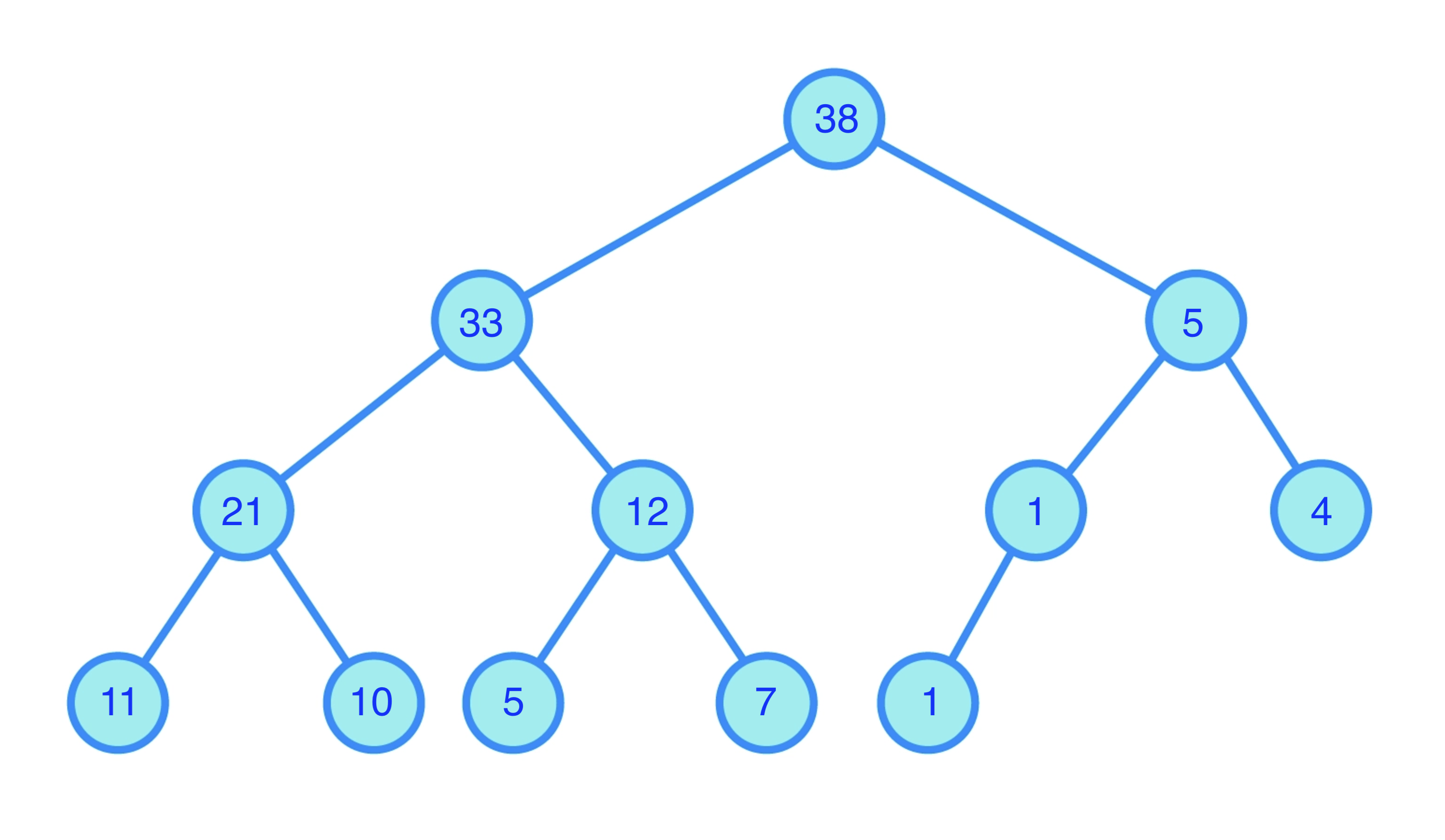Each tree supports maintenance of a collection of `k` real values (weights).
The `k` weights are assigned to the leaves
Each internal node has weight equal to the weights of the leaves of its subtree

Such a tree can be:

Updated (new weight added or changed) in `O(\log k)` time
Used to pick a weight `w_i` with probability `w_i/\sum_j w_j`.

Maintain a tree for each set of squared lengths:

Rows of `\mA`
Columns of `\mA`

(Sketch)

If `n\gt d`, work with the transpose, so WLOG `n\le d`.
The data structure is a collection of binary trees.

Using these trees, pick `\mS` and `\mR`
Obtain `\mZ` by applying `((\mA\mR)^\top\mA\mR)^+` to `(\mS\mA\mR)^\top`
Return `\mS`,`\mR`, and `\mZ`

Step 1 takes
`\quad O((m_S+m_R)\log(nd))` time;
Step 2 takes
`\quad O(n m_R^2)` to compute `(\mA\mR)^\top\mA\mR`,
`\quad O(m_R^3)` to compute the pseudo-inverse
`\qquad` (or matrices needed to apply the inverse)
`\quad O(m_R^2m_S)` to apply the pseudo-inverse.

Leverage-score sampling

More better variance reduction

Want sampler `\mS` so that `\norm{\mS\mA\vx}` is a good estimator of `\norm{\mA\vx}`

We've seen:

Uniform sampling: `p_i\propto\frac{1}{n}` might miss big rows
Length-squared (row) sampling: `p_i\propto \norm{\mA_{i*}}^2` is better,
but for some `\vx` maybe `\mA_{i*}\vx = 0` even if `\norm{\mA_{i*}}` is large

In either, maybe `\mA_{i*}\vx` is relatively large, and other entries of `\mA\vx` small
`\implies` large variance

We want the terms `(\frac{1}{\sqrt{p_i}}\mA_{i*}\vx)^2` to be "well-behaved"
for all `i` and `\vx`

Bounded sensitivity sampling

One sense of "well-behaved":
`\qquad\qquad` bounded relative contribution
The `i`th row contributes `(\mA_{i*}\vx)^2` to `\norm{\mA\vx}^2 = \sum_i (\mA_{i*}\vx)^2`

Suppose

unit `\vy\in\im \mA`
`\vtau\in\R^n` has `\tau_i \ge y_i^2` for `i\in [n]`
`\vs` is a sampling vector with distribution `\vp = \vtau/t`, where `t\equiv \sum_i \tau_i\ge\norm{\vy}^2`

Then as expected `\E[(\vs^\top\vy)^2] = \sum_i p_i \left(\frac{y_i}{\sqrt{p_i}}\right)^2 = \norm{\vy}^2`.

But also:

Larger entries of `\vy` are more likely to be picked
If `i` is picked, the estimate is `\left(\frac{y_i}{\sqrt{p_i}}\right)^2 = \frac{y_i^2}{\tau_i/t} \le t`.
So the estimate has a uniform upper bound of `t=\sum_i \tau_i`, always.

Extending from a sampling vector to a sampling matrix `\mS\in\R^{m\times n}`,
the estimate is a mean of `m` values, each bounded by `t`.
Using e.g. Bernstein's inequality, such estimates concentrate around their mean.

We want such a bounded effect for all `\vy\in\im\mA`, not just one.
This can be done by finding `\vtau` with `\tau_i\ge y_i^2` for all unit `\vy\in\im(\mA)`.

Leverage scores

Given linear subspace `L\subset\R^n`.
For `i\in[n]` the `i`'th leverage score `\tau_i(L)\equiv\sup_{\vy\in L} y_i^2/\norm{\vy}^2`.

Leverage scores of `\mA` The leverage scores of `\mA\in\R^{n\times d}` are `\tau_i(\mA) = \tau_i(\im(\mA))`.

Rows with a high score have more effect, more "leverage", on the least-squares fit.

Given matrix `\mA\in\R^{n\times d}`, and `\mU ` any orthonormal basis for `\im(\mA )`.
For `i\in[n]`, the `i`'th leverage score $$\tau_i(\mA) = \sup_{\vx} \frac{(\mA_{i*}\vx)^2 }{ \norm{\mA\vx}^2} = \norm{\mU_{i*}}^2.$$

For `L=\im(\mA) = \im(\mU)`, any `\vz\in L` has `\vz=\mA\vx=\mU\vy` for some `\vx` and `\vy`. We have

`\begin{align*} \sup_{\vx} \frac{(\mA_{i*}\vx)^2 }{ \norm{\mA\vx}^2} = \sup_{\vy} \frac{(\mU_{i*}\vy)^2 }{ \norm{\mU\vy}^2 } = \sup_{\vy} \frac{(\mU_{i*}\vy)^2 }{ \norm{\vy}^2 } = \norm{\mU_{i*}}^2. \end{align*}`

`\sum_i \tau_i(\mA) = \rank(\mA)`.
`\tau_i(\mA) \in [0,1]`.

Leverage-score sampling: concentration

Matrix Chernoff Let `\mX_k` for `k\in [m]` be i.i.d. copies of symmetric random `\mX\in \R^{d\times d}` with `\gamma,\sigma^2\gt 0`,
`\quad\E[\mX] = 0`,
`\quad\norm{\mX}_2 \le \gamma`, and
`\quad \norm{\E[\mX^2]}_2 \le \sigma^2`.
Then for `\eps\gt 0`,
`\qquad \Prob\{\norm{\frac1{m}\sum_k \mX_k}_2 \ge \eps\} \le 2d\exp(-m\eps^2/(\sigma^2 + \gamma\eps/3)).`

Derivable from Matrix Bernstein, e.g. Thm. 1.4 of [HT].

Given `\eps,\delta\gt 0` and `\mA\in\R^{n\times d}` with `r=\rank(\mA)`.
Construct a sampling matrix `\mS` using probabilities `p_i = \tau_i(\mA)/r`, so `\mS_{k*}=\ve_I/\sqrt{m p_I}` with `\Prob\{I=i\}=p_i`
There is `m = O(\eps^{-2}r\log(r/\delta))` so that `\mS` is an `\eps`-embedding of `\im(\mA)`, with failure probability `\delta`.

Let `\mU\in\R^{n\times r}` be orthonormal with `\im(\mU)=\im(\mA)`.
For `k\in[m]`, let `\mX_k = m\mU^\top[\mS_{k*}]^\top\mS_{k*}\mU - \Iden`, so `\frac{1}{m}\sum_k \mX_k = \mU^\top\mS^\top\mS\mU - \Iden`,
and for an `\eps`-embedding, we bound its spectral norm.
We apply matrix Chernoff to
`\mX = \frac{1}{p_I}[\mU_{I*}]^\top\mU_{I*} - \Iden` with `\Prob\{I=i\}=p_i=\tau_i(\mA)/r=\norm{\mU_{i*}}^2/r`.
We have:

`\E[\mX] = \E_I[\frac{1}{p_I}[\mU_{I*}]^\top\mU_{I*} - \Iden] = \mU^\top\mU - \Iden = 0`.
`\norm{\mX}_2 \le\max_I\frac{1}{p_I}\norm{[\mU_{I*}]^\top\mU_{I*}}_2 + \norm{\Iden}_2 = \frac{r}{\tau_I}\norm{\mU_{I*}}^2 + 1 = r + 1`.
`\begin{align*} \E[\mX^2] & = \E_I[\frac{1}{p_I^2}[\mU_{I*}]^\top\mU_{I*}[\mU_{I*}]^\top\mU_{I*}] -2\E_I[\frac{1}{p_I}[\mU_{I*}]^\top\mU_{I*}] + \Iden \\ & = \E_I[\frac{\tau_I}{p_I^2} [\mU_{I*}]^\top\mU_{I*}] - 2\mU^\top\mU + \Iden = r\Iden - 2\Iden + \Iden = (r-1)\Iden, \end{align*}`
so `\norm{\E_I[\mX^\top\mX]}_2 \le r-1`.

We can apply matrix Chernoff with `\gamma = r + 1` and `\sigma^2 = r-1`, obtaining
`\Prob\{\norm{\frac1{m}\sum_k X_k}_2 \ge \eps\} \le 2r\exp(- m\eps^2/((r-1) + (r + 1)\eps/3))`.
For `m = O(\eps^{-2} r\log(r/\delta))`, this is at most `\delta`.

Approximate scores

Sometimes sampling can only be done with probabilities that are only approximations to the leverage scores.

Given `\eps,\delta\gt 0,{\color{red}\alpha}\ge 1` and `\mA\in\R^{n\times d}` with `r=\rank(\mA)`.
Construct a sampling matrix `\mS` using probabilities `p_i \ge \tau_i(\mA)/({\color{red}\alpha} r)`, so `\mS_{k*}=\ve_I/\sqrt{m p_I}` with `\Prob\{I=i\}=p_i`
There is `m = O(\eps^{-2}{\color{red}\alpha} r\log(r/\delta))` so that `\mS` is an `\eps`-embedding of `\im(\mA)`, with failure probability `\delta`.

`\E[\mX] = \E[\frac{1}{p_I}[\mU_{I*}]^\top\mU_{I*} - \Iden] = \mU^\top\mU - \Iden = 0`.
`\norm{\mX}_2 \le\frac{1}{p_I}\norm{[\mU_{I*}]^\top\mU_{I*}}_2 + \norm{\Iden}_2 \le \frac{{\color{red}\alpha} r}{\tau_I}\norm{\mU_{I*}}^2 + 1 = {\color{red}\alpha} r + 1`.
`\begin{align*} \E[\mX^2] & = \E[\frac{1}{p_I^2}[\mU_{I*}]^\top\mU_{I*}[\mU_{I*}]^\top\mU_{I*}] -2\E[\frac{1}{p_I}[\mU_{I*}]^\top\mU_{I*}] + \Iden \\ & = \E[\frac{\tau_I}{p_I^2} [\mU_{I*}]^\top\mU_{I*}] - 2\mU^\top\mU + \Iden \le {\color{red}\alpha} r\Iden - 2\Iden + \Iden = ({\color{red}\alpha} r-1)\Iden, \end{align*}`
so `\norm{\E[\mX^\top\mX]}_2 \le {\color{red}\alpha} r-1`.

We can apply matrix Chernoff with `\gamma = {\color{red}\alpha} r + 1` and `\sigma^2 = {\color{red}\alpha} r-1`, obtaining
`\Prob\{\norm{\frac1{m}\sum_k X_k}_2 \ge \eps\} \le 2r\exp(- m\eps^2/(({\color{red}\alpha} r-1) + ({\color{red}\alpha} r + 1)\eps/3))`.
For `m = O(\eps^{-2} {\color{red}\alpha} r\log(r/\delta))`, this is at most `\delta`.

Friends and relations

Isotropic position:

If `\mU` has orthonormal columns,
its rows are in isotropic position
e.g., `\mA\mR^{-1}`, where `\mA=\mQ\mR`
Leverage score sampling == length-squared sampling
for matrix with rows in isotropic position.
As applied to volume of convex bodies,
coresets for Minimum Enclosing Ellipsoids;
coresets==small subsets with about the same MEE

Also:

Diagonal of hat matrix (influence matrix, projection matrix)
Spectral sparsification & effective resistance
Regression, and extension to `\ell_p`
Low-rank approximation: robust, and CUR
Sensitivity, more generally
- `\equiv` max relative cost of loss `i`, over all `\vx`
- High sensitivity == one definition of "outlier"

Computing leverage scores

Roughly: use sketch to get `\approx`orth. basis, use its row norms
(Same pre-conditioner scheme as for regression)

Given

Input matrix `\mA `
subspace `\eps`-embedding matrix `\mS\in\R^{m\times n}` for `\mA `
embedding (JL) matrix `\mathbf{\Pi}\in\R^{d\times m'}`,
so `\norm{\vx^\top\mathbf{\Pi}}=(1\pm\eps)\norm{\vx }` for `n` vectors `\vx `
- `m'=O(\eps^{-2}\log n)`

The algorithm:

`\mW = \mS *\mA `;	// compute sketch
`[\mQ,\mR ] = \mathtt{qr}(\mW )`;	// compute change-of-basis for `\mS\mA `
`\mZ = \mA (\mR^{-1}\mathbf{\Pi})`;	// compute sketch of `\mA\mR^{-1}`
return `\mathtt{dot}(\mZ,\mZ,2)`;	// return vector of squared row norms

Computing leverage scores: correctness

`\mA\mR^{-1}` has singular values `1\pm\eps`

For all `\vx`, `\norm{\mA\mR^{-1}\vx } \approx_\eps\norm{\mS\mA\mR^{-1}\vx } = \norm{\mQ\vx } = \norm{\vx }`

Let `\mU` be an orthonormal basis for `\im(\mA)`

`\mA\mR^{-1}` is "morally" like `\mU`,
pick `\mT` to translate, so that `\mA\mR^{-1}\mT = \mU`

`\mT ` has singular values `1\pm\eps`

For all `\vx`, `\norm{\mT\vx } = \norm{\mQ\mT\vx } = \norm{\mS\mA\mR^{-1}\mT\vx } \approx_\eps\norm{\mA\mR^{-1}\mT\vx } = \norm{\mU\vx } = \norm{\vx }`

`\mT^{-1}` has singular values `1\pm 2\eps` for `\eps\le 1/2`

The algorithm output `\norm{\ve_i^\top\mA\mR^{-1}\mathbf{\Pi}}^2 = (1\pm O(\eps)) \norm{\ve_i^\top\mU }^2`

`\norm{\ve_i^\top\mA\mR^{-1}\mathbf{\Pi}}\approx_\eps\norm{\ve_i^\top\mA\mR^{-1}} = \norm{\ve_i^\top\mU\mT^{-1}}\approx_{2\eps}\norm{\ve_i^\top \mU }`

Computing leverage scores: running time

`\mW = \mS *\mA `;	// `O(\nnz{\mA }s)` when `\mS ` is a sparse embedding, param `s`
`[\mQ,\mR ] = \mathtt{qr}(\mW )`;	// `O(d^2m)`
`\mZ = \mA (\mR^{-1}\mathbf{\Pi})`;	// `O(d^2m') +O(\nnz{\mA }m')`
return `\mathtt{dot}(\mZ,\mZ,2)`;	// `O(nm')`

Grand total, for `s=O(1/\eps)`, `m =O(d^{1+\gamma}/\eps^2)` [NN] $$\begin{align*} O(\nnz{\mA }(m'+s) & + O(d^2(m+m') \\ & = O(\nnz{\mA}\eps^{-2}\log n) + O(d^2\eps^{-2}(\log(n) + d^{1+\gamma}))\end{align*}$$

Or, use `s=O(\eps^{-1}\log d)`, `m=O(\eps^{-2}d\log d)` [Coh]

Leverage scores, finis

Given `\mA\in\R^{n\times d}` and `\eps\gt 0`, the leverage scores of `\mA` can be computed with relative error `\eps` in $$O(\nnz{\mA}\eps^{-2}\log n) + O(d^2\eps^{-2}(\log(n) + d\log d))$$ expected time.

Constant `\eps` is good enough for many purposes, such as leverage score sampling

For sampling, sometimes can make `m'=O(1/\eps^2)`
very crude estimates, but still good enough
(Maybe use `s=O(1/\eps)` to remove all logs in leading term)

Subsampled Randomized Hadamard Transform

SRHT: the Subsampled Randomized Hadamard Transform

In the original JL:
- Pick random orthogonal matrix `\mQ `
- Sketching matrix `\mS\equiv` the first `m` rows of `\mQ `
- `O(mnd)` time to compute `\mS\mA `
A faster scheme: pick a random orthogonal matrix, but:
- Use fewer random bits
- Make it faster to apply

This is "Fast JL", here we discuss a variant

The SRHT is a matrix `\mP\mH\mD`, applied on the left, where:

`\mD\in\R^{n\times n}` is diagonal with i.i.d. `\pm 1` on diagonal
`\mH\in\R^{n\times n}` is a Hadamard matrix (orthogonal, fast multiply)
`\mP\in\R^{m\times n}` uniformly samples rows of `\mH\mD`

`\qquad\qquad\small{ \underbrace{\left[\begin{matrix} 0 & 0 & 0 & \cdots & 1 \\ 1 & 0 & 0 & \cdots & 0 \\ 0 & 0 & 1 & \cdots & 0 \end{matrix}\right]}_\mP \underbrace{\left[\begin{matrix} 1 & 1 & 1 &\cdots & 1 \\ 1 & -1 & 1 &\cdots & -1\\ 1 & 1 & -1 &\cdots & -1\\ \vdots & \vdots & \vdots & \cdots & \vdots \\ 1 & -1 & -1 &\cdots&1 \\ \end{matrix}\right]}_{\sqrt{n}\mH} \underbrace{\left[\begin{matrix} \pm 1 & 0 & 0 &\cdots & 0 \\ 0 & \pm 1 & 0 &\cdots & 0\\ 0 & 0 & \pm 1 &\cdots & 0\\ \vdots & \vdots & \vdots & \ddots & \vdots \\ 0 & 0 & 0 &\cdots& \pm 1 \\ \end{matrix}\right]}_\mD } `

Hadamard: definition

Hadamard matrices have a recursive construction

Let `\mH_0\in\R^{1\times 1}` be the matrix `[1]`.
Let `\mH_{i+1}\equiv\frac{1}{\sqrt{2}}\left[\begin{matrix}\mH_i & \mH_i\\\mH_i & -\mH_i\end{matrix}\right]` for `i\ge 0`

So $$ \begin{align*} \mH_1 & \equiv\frac{1}{\sqrt{2}}\left[\begin{matrix} 1 & 1\\ 1 & -1\end{matrix}\right], \mH_2 = \frac{1}{2}\left[\begin{matrix} 1 & 1 & 1 & 1\\ 1 & -1 & 1 & -1\\1 & 1 & -1 & -1\\1 & -1 & -1 & 1\\\end{matrix}\right] \end{align*} $$

In general, `\mH_k` is `2^k\times 2^k` matrix of `\pm 1`, scaled by `1/2^{k/2}`

Hadamard: properties

Hadamard matrices `\mH_i` have `\mH_i^\top\mH_i=\mH_i^2 = \Iden`.

$$\mH_{i+1}^\top\mH_{i+1} = \mH_{i+1}^2 = \frac12\left[\begin{matrix}\mH_i & \mH_i\\\mH_i & -\mH_i\end{matrix}\right]\left[\begin{matrix}\mH_i & \mH_i\\\mH_i & -\mH_i\end{matrix}\right] = \frac12\left[\begin{matrix}2\mH_i^2 & \mH_i^2 -\mH_i^2\\\mH_i^2 -\mH_i^2 & 2\mH_i^2\end{matrix}\right] = \Iden$$

`\mH\vx` can be computed in `O(n\log n)`, for `x\in\R^n`, `n=2^k`.

Suppose `\vx =\left[\begin{smallmatrix} \vx' \\ \vx''\end{smallmatrix}\right]\in\R^{2^k}`,
where `\vx ',\vx ''\in\R^{2^{k-1}}`.

Then `\mH_{i+1}\vx =\left[\begin{smallmatrix} \mH_i \vx' +\mH_i\vx'' \\ \mH_i\vx' - \mH_i\vx''\end{smallmatrix}\right]`,
so `\mH_{i+1}\vx` found in linear time from `\mH_i\vx'` and `\mH_i\vx''`

Analysis of Fast Hadamard

Via the "flatness" of the leverage scores:

Flatness of leverage scores For `\mA,\mD, \mH` as above, $$\tau_i(\mH\mD\mA) \le \frac{d}{n}\left(1+\sqrt{8\log(n/\delta)/d}\right)^2$$ for all `i\in [n]`, with failure probability `\delta`.

Note that `\sum_{i\in [n]} \tau_i = d`, so average is `d/n`.

Next slide.

`\mP\mH\mD\mA ` can be computed in `O(nd\log n)` time.
There is $$m = O(d\eps^{-2}\log(d/\delta)\left(1+\sqrt{8\log(n/\delta)/d}\right)^2)$$ so that with failure probability `\delta`, `\mP\mH\mD ` is an `\eps`-embedding of `\im(\mA )`.

Apply flatness and approximate leverage score sampling result: uniform sampling of `\mP` is a fraction of `\tau_i/d` equal to
`\frac{1/n}{\tau_i/d} \ge \frac{1}{(1+\sqrt{8\log(n/\delta)/d})^2}`

Flatness of leverage scores of `\mH\mD\mA`

Concentration of convex functions of Rademachers [Led97] Suppose `f(\vx)` is a convex `L`-Lipschitz function,
so `f(\vx)-f(\vy) \le L\norm{\vx-\vy}`.
Then for `t\ge 0` and `\vr` a sign (Rademacher) vector, so `r_i=\pm 1` with equal probability, $$\Prob\{f(\vr) - \E[f(\vr)] \ge Lt\} \le \exp(-t^2/8).$$

`\E[f(\mD )]\le\sqrt{d/n}` Given `i\in[n]`, let `f(\mD )\equiv f_i(\mD) \equiv \norm{\mH_{i*}\mD\mA } = \sqrt{\tau_i(\mH\mD\mA)}`,
where `\mH,\mD,\mA` are as above.
Then `\E[f(\mD )]\le\sqrt{d/n}`.

Assume WLOG that `\mA` is orthonormal. Then $$(\mH\mD\mA )^\top\mH\mD\mA = \mA^\top\mD^\top\mH^\top\mH\mD\mA = \Iden,$$ so `f_i(D)^2 = \tau_i(\mH\mD\mA)`.
We have $$ \sum_i f_i(\mD)^2 = \sum_i \tau_i(\mH\mD\mA) = \rank(\mH\mD\mA) = d. $$ The random variables `\norm{\mH_{i*}\mD\mA }` have the same distribution, for all `i`,
so for any `i`, `\E[f_i(\mD)^2] = \frac1n\sum_{i'} \E[f_{i'}(\mD)^2] = \frac{d}n`,
and `\E[f(\mD )] \le \E[f(\mD)^2]^{1/2} \le \sqrt{d/n}`, using Jensen's inequality.

`f(\mD)` is convex and Lipschitz The function `f(\mD)` is convex and `\frac1{\sqrt{n}}`-Lipschitz.

Convex:
Since `\norm{\cdot}` is convex, and `\mH_{i*}\mD\mA` is a linear function of `\mD`, `f(\mD )\equiv\norm{\mH_{i*}\mD\mA }` is convex.

Lipschitz:
Let `\vm = [\mH_{i*}]^\top`. Then
`(\vm^\top\mD)_j = m_j d_{jj}`, or equivalently `d_j m_{jj}`, where `\vd` has `\mD=\diag(\vd)` and `\mM = \diag(\vm)`. That is,
`\vm^\top\mD = \vd^\top\mM`, and we could write `f(\mD)= \hat f(\vd) = \norm{\vd^\top\mM\mA}`.

We have
`\begin{align*} |\hat f(\vd) - \hat f(\vd')| & = |\,\norm{\vd^\top\mM\mA} - \norm{(\vd')^\top\mM\mA}\,| \\ & \le \norm{(\vd - \vd')^\top\mM\mA}& \text{ triangle inequality} \\ & \le \norm{\vd - \vd'}\,\norm{\mM}_2\norm{\mA}_2&\text{ Def. of spectral norm} \\ & = \frac{1}{\sqrt{n}}\norm{\vd - \vd'}\quad\implies \frac{1}{\sqrt{n}}\text{-Lipschitz} \end{align*}`

Flatness of leverage scores For `\mA,\mD, \mH` as above, $$\tau_i(\mH\mD\mA) \le \frac1{n}(\sqrt{d}+\sqrt{8\log(n/\delta)})^2$$ for all `i\in [n]`, with failure probability `\delta`.

Applying the concentration bound to `f(\mD)=\sqrt{\tau_i}`, and with the bound on `\E[f(\mD)]`,
`\Prob\{\sqrt{\tau_i}\ge \sqrt{d/n} + t/\sqrt{n} \} \le \exp(-t^2/8) = \delta/n`
for `t=\sqrt{8\log(n/\delta)}`; this implies the result,
taking a union bound over all `i\in[n]`.

Approximate Matrix Multiplication with SRHT

AMM with SRHT Given `\mA\in\R^{n\times d}`, `\mB\in\R^{d'\times n}`, `\eps\ge 0`.
There is `m=O(\eps^{-2}(\log(n/\delta)^2)` so that an SRHT `\mS=\mP\mH\mD\in\R^{m\times n}` has $$\norm{\mB\mS^\top\mS\mA - \mB\mA}_F \le \eps\norm{\mA}_F\norm{\mB}_F$$ with failure probability at most `\delta`.

Not given here; the bound is a little conservative.

Using SRHT to build a better `\mS `

Sparse embeddings take `O(\nnz{\mA })` to apply, but `m=O(d^2/\eps^2)`
Or `O(\nnz{\mA }/\eps)` to apply, with `m=O(d^{1+\gamma}/\eps^2)`.
- For sparse embeddings with `s\gt 1` nonzeros per column
Or: `O(\nnz{\mA }) +\tO(d^3/\eps^2)` to map to `m= \tO(d/\eps^2)`
- First apply a sparse embedding, then SHRT
- Subspace embeddings compose
- Matrix product approximators compose

Multiple-response
least-squares regression,
low-rank approximation

Fitting data: low-rank approximation

Fit: a `k`-dimensional subspace `L^*` minimizing $$\cost(\mA,L) \equiv \sum_{i\in [n]} \dist(\mA_{i*},L)^2$$ among all `k`-dimensional subspaces
That is, $$\min_{\substack{\mY\in\R^{n\times k}\\ \mX\in\R^{k\times d}}} \norm{\mY\mX - \mA}_F^2.$$
`\OPT` from Singular Value Decomposition (SVD) (PCA, LSI, EigenX,...)
For fixed `\mY`, least-squares for each column of `\mX`
For fixed `\mX`, least-squares for each row of `\mY`
Length-squared sampling gives a CUR decomposition.
We seek relative error approximation:
given `\eps\gt 0`, find `\tmY,\tmX` with $$\norm{\tmY\tmX - \mA}_F^2 \le (1+\eps)\OPT$$

Multiple-response regression

Let

`\mA\in\R^{n\times d}`
`\mB\in\R^{n\times d'}`

The multiple-response, or generalized, regression problem is to find $$\argmin_{\mX\in\R^{d\times d'}}\norm{\mA\mX -\mB}_F$$

Since $$\norm{\mA\mX -\mB}_F^2 = \sum_{j\in[d']}\norm{\mA\mX_{*j} - \mB_{*j}}^2,$$ no harder than `d'` independent least-squares problems.

But: using the same sketch for `d'` subspace embeddings doesn't (provably) work if failure probability is too large.

Countsketch: constant failure probability per right-hand-side ☹️
Leverage-score sampling
1. Exponentially small failure probability 😀
2. Not oblivious ☹️

We will use oblivious sketches for multiple-response regression
to do low-rank approximation.

Good regression sketches `\implies` weak coresets

Linear span containment For `\mA\in\R^{n\times d}`, let `\mY^*, \mX^* \equiv \argmin_{\substack{\mY\in\R^{n\times k}\\ \mX\in\R^{k\times d}}} \norm{\mY \mX - \mA}_F^2`.
Then `\mY^* = \mA(\mX^*)^+`, and `\mX^*=(\mY^*)^+\mA`
So `\mY^*= \mA\mW`, `\mX^*= \mH\mA` for some matrices `\mW` and `\mH^\top` with `k` columns.

Use the pseudo-inverse to solve the least-squares problems per-column.

Suppose `\mR` is good for multiple-response regression, that is,
`\quad\tmY \equiv \argmin_{\mY\in\R^{n\times k}} \norm{(\mY \mX^* - \mA)\mR}_F^2`
has
`\quad\norm{\tmY \mX^* - \mA}_F^2 \le (1+\eps)\norm{\mY^*\mX^*-\mA}_F^2`.
Then WLOG, `\tmY=\mA\mR\tmW` for some `\tmW` with `k` columns,
and
`\quad\norm{\mA\mR\tmW\mX^* - \mA}_F^2 \le (1+\eps)\norm{\mY^*\mX^*-\mA}_F^2`.

From just above, `\tmY = \mA\mR(\mX^*\mR)^+` solves the sketched version,
so `\tmW=(\mX^*\mR)^+` satisfies the conditions.

The columns of `\mA\mR` contain a left factor of a low-rank approximation: it is a weak coreset

Similar observations, applying sketching matrix `\mS` to `\min_{\mX\in\R^{k\times d}} \norm{\mA\mR\tmW \mX - \mA}_F^2`, yield the following.

Low-rank approximation: reduction to `\mA\mR\mZ\mS\mA`

Given `\mA\in\R^{n\times d}`,
`\mR` giving `\eps`-approximate solution `\mA\mR\tmW` to `\min_{\mY\in\R^{n\times k}} \norm{\mY \mX^* - \mA}_F^2`,
`\mS` giving `\eps`-approximate solution `\tmH \mS\mA` to `\min_{\mX\in\R^{k\times d}} \norm{\mA\mR\tmW \mX - \mA}_F^2`.
Then $$\tmW, \tmH \equiv \argmin_{\substack{\mW\in\R^{m_R\times k}\\\mH\in\R^{k\times m_S}}} \norm{\mA\mR\mW\mH\mS\mA - \mA}_F^2$$ gives rank-`k` matrix `\mA\mR\tmW\tmH \mS\mA` with `\norm{\mA\mR\tmW\tmH \mS\mA - \mA}_F \le (1+O(\eps))\min_{\rank(\mB)=k}\norm{\mB - \mA}_F`.

Letting `\mZ=\tmW\tmH`, the reduction looks like:

$$\begin{align*} \min_{\substack{\mY\in\R^{n\times k}\\ \mX\in\R^{k\times d}}} \norm{\mY & \mX - \,\, \!\!\mA }_F \\[-10em] & \Bigg\downarrow & \\[-9em] \min_{\rank(\mZ)=k} \norm{\mA\mR & \mZ\mS\mA - \mA}_F \end{align*}$$

TBD:

Finding oblivious sketching distributions "good for regression"
Solving the resulting problem

Least-squares regression, again: weaker conditions

Before:
`\mS ` a subspace `\eps`-embedding for `[\mA\ \vb]\implies`
`\argmin_{\vx\in\R^d}\norm{\mS (\mA\vx -\vb)}` `\eps`-approx for `\min_{\vx\in\R^d}\norm{\mA\vx -\vb}`

However, weaker conditions are enough:

`\mA\in\R^{n\times d}` with `\rank(\mA )=r`, `\vb\in\R^n`
`\mS ` with `\norm{\mW\mS^\top\mS\mW' - \mW\mW'}_F \le \frac23\sqrt{\eps/r}\norm{\mW}_F\norm{\mW'}_F` for fixed unknown `\mW ,\mW '`
`\mS ` a subspace `(1/9)`-embedding for `\mA `

Then for $$ \begin{align*} \tvx & \equiv\argmin_{\vx\in\R^d}\norm{\mS (\mA\vx -\vb)} \\\vx_* & \equiv\argmin_{\vx\in\R^d}\norm{\mA\vx -\vb}, \end{align*} $$ we have $$\norm{\mA\tvx -\vb}\le (1+\eps)\Delta_*,\text{ where }\Delta_*\equiv\norm{\mA\vx_*-\vb}$$

Proof:next couple slides

If for any fixed `\vy`,
`\qquad \norme{\norm{\mS^\top\mS-\Iden}_{\{\vy\}}}_{2} \le K\min\{\sqrt{\eps/r}, 1/r\}`
then the above conditions hold. A countsketch embedding to `O(r/\eps + r^2)` dimensions suffices.

An SRHT to `\tO(r/\eps)` dimensions suffices to satisfy the approximate matrix multiply and subspace embedding conditions above.

Proof, least squares from AMM + const-embedding, 1/2

We can assume WLOG `\mA ` has orthonormal columns
`\mS ` is a `(1/9)`-embedding $$\implies\norm{\mA^\top\mS^\top\mS\mA -\Iden}_2\le 1/3 \implies \sigma_\min(\mA^\top\mS^\top\mS\mA) \ge 2/3$$
The normal equations: $$\mA^\top (\mA\vx^* -\vb) = 0 = \mA^\top\mS^\top\mS (\mA\tvx -\vb)$$
Using the first normal eq. and by Pythagoras, $$\begin{align*} \norm{\mA\tvx-\vb}^2 & = \norm{\mA\tvx -\mA\vx^*}^2 +\norm{\mA\vx^*-\vb}^2\\ & = \norm{\tvx -\vx^*}^2 +\Delta_*^2 \end{align*}$$
- By (1), `\norm{\mA\vy }= \norm{\vy }`

So it is enough show that $$\norm{\tvx -\vx^*}\le\sqrt{\eps}\Delta_*.$$ (Note: this bound is for `\tvx,\vx^*` for `\mA` assumed orthonormal, that is, where an orthonormal basis is used for the analysis.)

Proof, least squares from AMM + const-embedding, 2/2

$$\begin{alignat*}{2} (2/3) & \norm{\tvx -\vx^*} & & \\ & \le \norm{\mA^\top \mS^\top\mS\mA (\tvx-\vx_*)} & & \,(\text{since }\sigma_\min(\mA^\top\mS^\top\mS\mA )\ge 2/3 ) \\ & = \norm{\mA^\top\mS^\top\mS (\mA\tvx -\mA\vx_*) \\ & \qquad\qquad -\mA^\top\mS^\top\mS (\mA\tvx -\vb) } & & \,(\text{normal eq. for sketched problem} ) \\ & = \norm{\mA^\top\mS^\top\mS (\vb -\mA\vx_*) } & & \\ & \le (2/3)\sqrt{\eps/r}\norm{\mA }_F\norm{\vb-\mA\vx^*} & & \,(\text{normal eq. for given problem, AMM bound} ) \\ & = (2/3)\sqrt{\eps}\Delta_*, & & \,(\rank(\mA )=r,\mA^\top\mA = \Iden ) \end{alignat*}$$

So $$\norm{\tvx -\vx^*}\le \sqrt{\eps}\Delta_*,$$ as claimed.

Multiple-response regression

Nearly the same proof as for 1-response regression shows:

`\mA\in\R^{n\times d}` with `\rank(\mA )=r`, `\mB\in\R^{n\times d'}`
`\mS ` with `\norm{\mW\mS^\top\mS\mW' - \mW\mW'}_F \le \frac23\sqrt{\eps/r}\norm{\mW}_F\norm{\mW'}_F` for fixed unknown `\mW ,\mW '`
`\mS ` a subspace `(1/9)`-embedding for `\mA `

Then for $$ \begin{align*} \tmX & \equiv\argmin_{\mX\in\R^{d\times d'}}\norm{\mS (\mA\mX -\mB)}_F \\\mX_* & \equiv\argmin_{\mX\in\R^{d\times d'}}\norm{\mA\mX - \mB}_F, \end{align*} $$ we have $$\norm{\mA\tmX-\mB}_F\le (1+\eps)\Delta_*,\text{ where }\Delta_*\equiv\norm{\mA\mX _*-\mB}_F$$

Same conditions on sketch as for 1-response
`\norm{\text{vector}}\rightarrow\norm{\text{matrix}}_F`
Pythagoras `\rightarrow` Matrix Pythagoras:
if matrices `\mA,\mB` have `\trace\mA^\top\mB=0`, then `\norm{\mA+\mB}_F^2 = \norm{\mA}_F^2 + \norm{\mB}_F^2`

If for any fixed `\vy`, $$\norme{\norm{\mS^\top\mS-\Iden}_{\{\vy\}}}_{2} \le K\min\{\sqrt{\eps/r}, 1/r\},$$ then the above conditions hold.
A sparse embedding to `O(r/\eps + r^2)` dimensions suffices.

These imply the conditions on `\mS` needed above.

An SRHT to `\tO(r/\eps)` dimensions suffices to satisfy the approximate matrix multiply and subspace embedding conditions above.

Low-rank approximation

Putting this construction for multiple-response regression with
the reduction of low-rank approximation,

Given `\mA\in\R^{n\times d}`,
there is sketching distribution `\mR\in\R^{d\times m_R}`
and sketching distribution `\mS\in\R^{m_S\times n}`, with `m_R,m_S=O(k/\eps + k^2)`, so that with constant failure probability `\begin{equation}\label{eq LRA}\tmZ \equiv \argmin_{\mZ:\rank(\mZ)=k} \norm{\mA\mR\mZ\mS\mA - \mA}_F^2 \end{equation}` gives rank-`k` matrix `\mA\mR\tmZ \mS\mA` with
$$\norm{\mA\mR\tmZ \mS\mA - \mA}_F \le (1+O(\eps))\min_{\rank(\mB)=k}\norm{\mB - \mA}_F.$$

First use the reduction of LRA to matrix multiplication and subspace embedding,
and then the reduction of the latter to the single vector case,
and then conditions on sparse embeddings for the single vector case.

Note that in the reduction from LRA,
`\rank(\mX^*)=\rank(\mA\mR\tmW)=k`,
so `m_R, m_S=O(k/\eps + k^2)` suffice.

It remains to solve `\eqref{eq LRA}`.
We can further reduce the problem size using... more sketching: affine embeddings.

Affine embeddings

Affine embeddings are like subspace embeddings, but "translated by `\mB `"

Given `\mA\in\R^{n\times d},\mB\in\R^{n\times d'}`, a matrix `\mT ` is an affine embedding for `\mA ,\mB ` if $$\norm{\mT (\mA\mX -\mB)}_F^2 = (1\pm\eps)\norm{\mA\mX -\mB }_F^2$$ for all `\mX\in\R^{d\times d'}`.

Note that since the condition applies for all `\mX`,
it applies in `\min_{\mZ:\rank(\mZ)=k}\norm{\mA\mR\mZ\mS\mA - \mA}_F^2` to `\mX` of the form `\mZ\mS\mA`.

Affine embeddings need a bit more from sketching matrices:

`\mA\in\R^{n\times d}` with `\rank(\mA )=r`, `\mB\in\R^{n\times d'}`
`\mT` with `\norm{\mW\mT^\top\mT\mW' - \mW\mW'}_F \le K_1\eps/\sqrt{r}\norm{\mW}_F\norm{\mW'}_F`
for fixed unknown `\mW ,\mW '`, constant `K_1`
`\mT ` a subspace `K_2\eps`-embedding for `\mA `, constant `K_2`

Then
`\mT ` is an affine `\eps`-embedding for `\mA ,\mB `, when `K_1` and `K_2` are small enough.

Low-rank approximation: the final sketching reduction

Now we pick affine embedding sketching matrices `\mS_\ell\in\R^{m_\ell\times n}` and `\mS_r\in\R^{d\times m_r}`, so our reduction is:

$$\begin{align*} \min \norm{\mA - \,\, & \!\!\mY \mX }_F \\[-10em] & \Bigg\downarrow & \\[-10em] \min_{\rank(\mZ)=k} \norm{\mA - \mA\mR & \mZ \mS\mA}_F \\[-10em] & \Bigg\downarrow & \\[-40em] \min_{\rank(\mZ)=k} \norm{ \mS_\ell (\mA - \mA\mR & \mZ \mS\mA) \mS_r}_F \end{align*}$$

Note that the reduced problem involves matrices `\mS_\ell\mA\mS_r`, `\mS_\ell\mA\mR`, `\mS\mA\mS_r` of dimensions `\poly(k/\eps)`

Low-rank approximation: overall

Assuming the reduced problem can be solved in `\poly(k/\eps)` time, we have:

Given `\mA\in\R^{n\times d}`, `\eps>0`, target rank `k`.
There is a construction that with constant failure probability finds `\mA\mR\in\R^{n\times m_R}, \mS\mA\in\R^{m_S\times d}`, `\tmZ\in\R^{m_R\times m_S}` of rank `k`, where `m_R,m_S=O(k/\eps + k^2)`
such that `\norm{\mA\mR\tmZ\mS\mA - \mA}_F\le (1+\eps)\min_{\mB:\rank(\mB)=k} \norm{\mB - \mA}_F`,
taking time `\tO(\nnz{\mA}) + O(n+d)\poly(k/\eps) + \poly(k/\eps).`

What's left is mainly the running time:

`\tO(\nnz{\mA})` for sketching
`\poly(k/\eps)` to solve small-matrix problem (a low-rank approx problem)
`O(n+d)\poly(k/\eps)` to compute `\mA\mR\tmY` and `\tmX\mS\mA`,
where `\tmZ=\tmY\tmX`, and `\tmY` and `\tmX^\top` have `k` columns

For completeness, how the small problem can be solved:

Generalized low-rank approximation[FT07] Given `\mA\in\R^{n\times d}`, `\mB\in\R^{n\times n_B}`, `\mC\in\R^{n_C\times d}`.
The Generalized Low-Rank Approximation problem is $$\min_{\textrm{rank}(\mX)= k} \|\mA - \mB \mX \mC \|^2_F,$$ and one solution is $$\mX = \mB^+[\mP_\mB \mA \mP_{\mC^\top}]_k \mC^+,$$ where `\mP_{\mB},\mP_{\mC^\top}` are the projection matrices onto `\im(\mB)` and `\im(\mC^\top)` respectively. Here `[\mW]_k` denotes the best rank-`k` approximation to `\mW`.

Low-rank approximation: regularization

Regularization $$\norm{\mY\mX-\mA}_F^2 \color{red}{+ \lambda(\norm{\mY}_F^2 + \norm{\mX}_F^2)}$$ just adds sketched regularizers.

Reduction to `\poly(k/\eps)` regularized problem
$$\tmW, \tmZ \equiv \argmin_{\mW,\mZ} \norm{\hmS \mA\mR\mW\mZ\mS\mA \hmR - \hmS A \hmR}_F^2 \color{red}{+ \lambda(\norm{\hmS\mA\mR\mW}_F^2 + \norm{\mZ\mS\mA\hmR}_F^2)}$$ gives rank-`k` matrix `\mA\mR\tmW\tmZ \mS\mA` with cost `(1+O(\eps))\OPT`

Using orthogonal invariance of `\norm{\cdot}_F`
reducible to regularized low-rank approximation.

Don't need much more for regularizer `F(\mY,\mX)`:

`F(\cdot,\cdot)` is subadditive in each argument
`F(\mY,\mX) = F(\mU\mY, \mX\mV)` for all orthogonal `\mU,\mV`, and
`F(\mY,\mX) = F\left(\left[\begin{smallmatrix}\mY & \mZero \\ \mZero & \mZero \end{smallmatrix}\right], \left[\begin{smallmatrix} \mX & \mZero \\ \mZero & \mZero \end{smallmatrix}\right]\right)`

So for example `F(\mY,\mX) = \min\{\norm{\mY^\top}_{2,1} + \norm{\mX}_{2,1}, \norm{\mY\mX}_*^{1/2} \}.`
(Where `\norm{\mE}_{2,1} \equiv \sum_i \norm{\mE_{i*}}_2`)

LASSO not included

Ridge regression

Work for some regularized problems can be provably less

Ridge regression: $$\min_{\vx\in\R^d} \norm{\mA\vx - \vb}^2 + \lambda\norm{\vx}^2,$$ Sketched version: $$\min_{\vx\in\R^d} \norm{\mS(\mA\vx - \vb)}^2 + \lambda\norm{\vx}^2.$$

When `\lambda` is very large, `\lambda\norm{\vx}^2` dominates, and
`\norm{\mS(\mA\vx - \vb)}^2 = (1+\eps) \norm{\mA\vx - \vb}^2` can have larger `\eps`.

So ridge regression should get easier as `\lambda` increases.

How much easier?

The statistical dimension of ridge regression

The statistical dimension (regression degrees of freedom, effective dimension) of ridge regression is $$ \sd_\lambda(\mA) \equiv \sum_i \frac{1}{1+\lambda/\sigma^2_i(\mA)},$$ where `\sigma_i(\mA)` is the `i`'th singular value of `\mA`.

Note that
`\sd_\lambda(\mA)\le \rank(A)\le \min\{n,d\}`, and
`\sd_\lambda(\mA)` is decreasing in `\lambda`.

Relates to sample complexity, ridge leverage scores

Not the one related to Gaussian width, or others

Smaller embeddings for ridge regression

A ridge regression problem with `n` rows can be reduced to one with
`\tO(\eps^{-1}\sd_\lambda(\mA))` rows, in
`O(\nnz{\mA}) + \tO(d\sd_\lambda(\mA)(\eps^{-1} + \sd_\lambda(\mA)))` time.
The resulting problem yields a `(1+\eps)`-approximation.

This are also similar results with `\sd` for sampling
Similarly for low-rank approximation; some `k\rightarrow O(\eps^{-1}\sd_\lambda(\mY_*))`
There is another reduction that reduces `d` to $$\poly(\sd_\lambda(\mA) \eps^{-1} (\sigma_1(\mA)^2/\lambda))$$
Contrast with "truncated optimization `\equiv` regularization" [MO11]

Low-rank approximation: robust

Suppose $$\mY^*, \mX^* \equiv \argmin_{\substack{\mY\in\R^{n\times k}\\{\mX\in\R^{k\times d}}}} \norm{\mY \mX - \mA}_{2,1}^2$$

Where `\norm{\mE}_{2,1} \equiv \sum_i \norm{\mE_{i*}}_2`; more generally `\norm{\mE}_M \equiv \sum_i M(\norm{\mE_{i*}}_2)` for `M(\cdot)`

As before, `\mY^*= \mA\mW`, `\mX^* = \mZ\mA` for some `\mW,\mZ`
For `\mX^*`, follows as before; for `\mY^*`, because `\mY^* = \mA(\mX^*)^+`

Can sketch on the right, since `\norm{\mE_{i*}\mR}_2 = (1\pm\eps)\norm{\mE_{i*}}_2`,
reduce to `\min_{\mW\in\R^{m\times k}, \mX\in\R^{k\times d}} \norm{\mA\mR\mW\mX - \mA}_M`
But: need new proof that `\mR` gives good approximate solution

Also: need subspace embedding `\mS` on the left, so that `\norm{\mS\mA\mR\mW\mX}_M \approx \norm{\mA\mR\mW\mX}_M`.

Construct `\mS` to sample rows of `\mA\mR`,
use `\eps`-net arguments in `\norm{\cdot}_M` space

Leverage score sampling of `\mA\mR` `\rightarrow` constant factor solution `\rightarrow` residual sampling `\rightarrow` `(1+\eps)` solution

Oblivious sketches: Sub-Gaussian Matrices

SubGaussian matrices

We've looked at sketching matrices
`\mS\in\R^{m\times n}` with `\E[s_{ij}]=0` and `\Var[s_{ij}]=1/m`,
and shown that when `s_{ij}` is Gaussian, `\mS` is an `\eps`-embedding with high probability.

Here we consider sketching vectors and matrices with random entries satisfying the sub-Gaussian condition (defined shortly).

A sub-Gaussian sketching vector or matrix has independent sub-Gaussian entries

As discussed next, for sub-Gaussian sketching vector `\vs`, sub-Gaussian sketching matrix `\mS`, and vector `\vy`:

`\vs^\top\vy `, a weighted sum of sub-Gaussians, is also sub-Gaussian
`(\vs^\top\vy )^2` is a sub-exponential random variable
`\norm{\mS\vy }^2` is :
- Also sub-exponential
- Concentrated

Sub-Gaussians as generalizations

Gaussian random variables have many interesting and useful properties, in particular, small "tails".
Sub-Gaussians are random variables with tails as small as Gaussians.

A random variable with a sub-Gaussian distribution,
denoted `X\sim\subg(\sigma_X^2)`, has a parameter `\sigma_X`, the variance proxy.

Below, relations for
Gaussians: `X\sim\cN(0,\sigma^2)`, and independent `X_i\sim\cN(0,\sigma^2)`, and for
Sub-Gaussians: centered `X\sim\subg(\sigma_X^2)`, and centered independent `X_i\sim\subg(\sigma_X^2)`
("Centered" means `\E[X]=0`)

`\begin{align*} && && \text{Gaussian} && \text{Sub-Gaussian}\\ \text{Tails} && \log \Prob\{|X|\ge t\} && \le \ln(2)-t^2/2\sigma^2 && \le 1-C_1t^2/2\sigma_X^2 \\ \text{Moments}, p\ge 1 && \norme{X}_p/\sqrt{p}, && \le \sigma && \le C_2\sigma_X\\ \psi_2\text{ norm} && \norme{X}_{\psi_2}, && \le \sigma && \le C_2\sigma_X\\ \text{Weighted sums} && \sum_i a_iX_i && \sim\cN(0,\sigma^2\norm{\va}^2) && \sim\subg(C_3\sigma_X^2\norm{\va}^2)\\ \text{Cumulant GF} && \log\E[\exp(tX)] && = t^2\sigma^2/2 && \le t^2\sigma_X^2/2 \\ \text{Sums of squares} && \sum_i X_i^2 && \chi\text{-squared} && \text{sub-exponential} \end{align*}`

The `C_i` and `K` are absolute constants

Cumulant generating functions

cumulant generating functions `\cgf_X(t)`
The cumulant generating function of real random variable X is
`\cgf_X (t) = \log\E[\exp(tX)]`, for `t\in\R`
It holds that
`\cgf_X(t) = \E[X]t +\frac12\Var[X]t^2 +\sum_{i>2}\frac1{i!}\kappa_i t^i\ldots`
where for `i\ge 1`, `\kappa_i` is the `i`th cumulant

(Gaussian) If `X\sim N(0,1)`, then `\cgf_X(t) = \frac12t^2`
(Sign) If `X= \pm 1` with equal probability, `\cgf_X(t) = \log((\exp(t) +\exp(-t))/2) = \log\cosh(t)`

additivity of `\cgf` If `X` and `Y` are independent, then `\cgf_{X+Y}(t) = \cgf_X(t) +\cgf_Y(t)`

Sub-Gaussians

`X` sub-Gaussian`\iff` there is a variance proxy `\sigma_X^2` with `\cgf_{X-\E[X]}(t)\le\sigma_X^2 t^2/2` for all `t`

(Gaussian) If `X\sim N(0,\sigma^2)` , `\sigma_X^2= \sigma^2`
(Sign) If `X= \pm 1` with equal prob., `\frac{e^t + e^{-t}}{2}\le e^{t^2/2}\implies \cgf_X(t) = \log\cosh(t)\le t^2/2`, so `\sigma_X^2=1`
(Bounded) If `|X|\le M` for some `M`, then `\cgf_{X-\E[X]} (t)\le M^2t^2/2`, so `\sigma_X^2\le M^2`

If `X` is centered sub-Gaussian, `\cgf_{\alpha X}(t) = \cgf_X (\alpha t)\le\sigma_X^2\alpha^2 t^2/2`

If `\vs` is a sub-Gaussian sketching vector with `\sigma\equiv \max_{i\in [n]} \sigma_{s_i}`,
then `\cgf_{\vs^\top\vy }(t) = \sum_{i\in [n]}\cgf_{s_i y_i}(t)\le\sum_{i\in [n]}y_i^2\sigma^2 t^2/2\le\sigma^2\norm{\vy }^2t^2/2`
That is, `\vs^\top\vy ` is sub-Gaussian with `\sigma_{\vs^\top\vy}^2 \le \sigma^2\norm{\vy }^2`
(Recall that `\Var(\vs^\top\vy) = \sigma^2\norm{\vy}^2` under analogous conditions.)

Concentration for sketching vectors

For centered real random variable `X`,
and for any value `t`, $$\log \Prob\{X\ge\alpha\} \le -t\alpha + \log \E[\exp(tX)].$$

If `Y\ge 0` then for `C\gt 0`, `\Prob\{Y\ge C\}\le\E[Y]/C`.
Letting `Y= \exp(tX)` and `C= \exp(t\alpha)` for `\alpha,t\ge 0`, with `X` centered, `\Prob\{X\ge\alpha\} = \Prob\{\exp(tX)\ge\exp(t\alpha)\}\le\E[\exp(tX)]\exp(-t\alpha)`

If `X` is sub-Gaussian then `\,\log\Prob\{X\ge\alpha\} \le -\alpha^2/2\sigma^2_X.`

If `X` is sub-Gaussian then
`\begin{align*} \log\Prob\{X\ge\alpha\} & \le\inf_{t\ge 0} -t\alpha +\cgf_X(t) \\ & = - \sup_{t\ge 0} t\alpha -\cgf_X(t) \le -\alpha^2/2\sigma^2_X. \end{align*}`

(Irrelevant fun fact: that `\sup` is the convex conjugate (a.k.a. Legendre-Fenchel transform) of `\cgf_X(t)`)
Putting this together with the CGF of a linear combination, a "Hoeffding-like":

If `\vs` is a sub-Gaussian sketching vector with `\sigma_{s_i}^2\le\sigma^2` for `i\in [n]`, then $$\Prob\{\vs^\top\vy\ge\beta\} \le \exp(-\beta^2/2\sigma^2\norm{\vy}^2).$$

Concentration for sketching matrices, 1/4

But:

We want to have an estimate closer to `\norm{\vy }`
We need even yet more concentration

We turn back to `\mS\in\R^{m\times n}`, a stack of sketching vectors
The summands in `\norm{\mS\vy }^2 = \sum_{j\in[m]} (\mS_{j*}\vy )^2` are sub-exponential:

`X^2` is sub-exponential `\iff` `X` is sub-Gaussian

So, the tail of `Y=X^2` decays "only" exponentially:
`\log\Prob\{Y\ge\beta\}\le -\beta/2\sigma^2_X`

Concentration for sketching matrices, 2/4

For small `t`, the `\cgf` of a centered sub-exponential looks like that of a centered sub-Gaussian:

sub-exponential CGF bound (NPH) if `Y=X^2-\E[X^2]` for sub-Gaussian `X`, then $$\cgf_Y(t)\le K_1 t^2\sigma_{X}^4$$ when `|t|\le K_2 /\sigma^2_X`, for constants `K_1` and `K_2`

Concentration for sketching matrices, 3/4

A "Bernstein-like" tail estimate for sums of sub-exponentials:

If `X_i`, for `i\in [m]`, are independent centered sub-Gaussian with `\sigma_{X_i}^2\le\sigma^2/m` and `\E[X_i^2] = 1/m`, then `Z= \sum_{i\in [m]} X_i^2` has $$Z\approx_\eps \E[Z]=1$$ with failure probability at most $$2\exp(-K_3 m\min\{\eps^2/\sigma^4,\eps/\sigma^2\}),$$ for a constant `K_3`.

When `|t|\le K_2/\sigma^2`, $$\cgf_{Z-\E [Z]}(t) = \sum_{i\in[m]}\cgf_{X_i^2-\E [X_i^2]}(t)\le K_1 t^2\sigma^4/m,$$ So
`\begin{align*} \log\Prob\{Z-\E[Z]\ge\alpha\} & \le\inf_{t\in [0,K_2m/\sigma^2] } -t\alpha + K_1 t^2\sigma^4/m, \\ & = -\min\{m\alpha^2/4K_1\sigma^4, m\alpha K_2/2\sigma^2\} \end{align*}`
Now let `\alpha= \eps\E[Z] = \eps`. Bounding also for `-Z`, and a union bound, gives the result.

Concentration for sketching matrices, 4/4

Translated to sketching matrices,

Fix unit `\vy\in\R^n`. Let `\mS\in\R^{m\times n}` with i.i.d. sub-Gaussian entries, and with `\E[\norm{\mS\vy }^2] = 1` and `\sigma_{\mS_{ij}}^2\le C/m` for a constant `C`. Then $$\norm{\mS\vy }^2=1\pm\eps$$ with failure probability at most $$2\exp(-K m\eps^2 ),$$ for a constant `K`.

That is, independent sub-Gaussian entries yield sketching matrices so that with very high probability, the norm of a single vector is preserved.

Distances

With the concentration results, the conclusions for sketching distances and subspaces follow, as for Gaussians.

For distances among points in `\cP\subset\R^n`, we can apply the concentration results to all vectors in `\cP-\cP=\{\vx-\vy\mid \vx, \vy\in\cP\}`

We have:

Let `\mS\in\R^{m\times n}` have

i.i.d. sub-Gaussian entries
`\E[\norm{\mS\vy }^2] = \norm{\vy}^2` for fixed `\vy\in\R^n`
`\sigma_{\mS_{ij}}^2\le C/m` for a constant `C`.

For given `\cP\subset \R^n`, there is a constant `K` and `m\le 2K\eps^{-2}\log(2|\cP|)` such that `\norm{\symd{\mS}}_{\cP-\cP} \le \eps` with probability at least `1/2`.

Subspace Embedding

Given `\delta, \eps\gt 0`, let `\mS\in\R^{m\times n}` have

i.i.d. sub-Gaussian entries
`\E[\norm{\mS\vy }^2] = \norm{\vy}^2` for fixed `\vy\in\R^n`
`\sigma_{\mS_{ij}}^2\le C` for a constant `C/m`.

For `\mA\in\R^{n\times d}`, there is `m=O(\eps^{-2}d\log(1/\delta))` so that with failure probability at most `\delta`,
`\mS ` is an `\eps`-embedding for `\im(\mA )`.

Use sketching matrix concentration, and the result showing that i.i.d. sketching matrices yield an embedding with high probability.

Slides for SLMath Summer School The Mathematics of Big Data: Sketching and (Multi-) Linear Algebra (Slides on matrix sketching) Ken Clarkson IBM Research

Introduction, Algorithmic Motivation

Outline

Outline

Regression

Least squares is still important

(Some) notation and conventions

Low-rank approximation: fitting data

Randomized approximation

Linearity of expectation, Markov's inequality, and union bounds

Product and norm estimation using randomization

Algorithms

`\eps`-approximations

Sketching Matrices: Oblivious Subspace Embeddings

Sketch and solve

Subspace embeddings for sketch and solve

Good sketching matrices

Algorithmic problems beyond regression

A sample of other uses of sketching

More `\tO(\nnz{\mA})`, not using sketching

Extension: kernelization

Extension: robustness

Extension: regularization

Course outline

Some basics

Orthonormal matrices, projection

The singular value decomposition

Eigendecomposition

The normal equations, the Moore-Penrose pseudo-inverse

The `QR` decomposition

The spectral norm and eigenvalues

The trace

Norms !

Some norms: matrices

Some norms: random variables

Matrix norms from sets: relation to spectral norms and embedding

From `\norm{\mW}_\cN` to `\norm{\mW}_2`: `\eps`-nets

`\norm{\mW}_{\cN_\eps}\approx\norm{\mW}_\cS = \norm{\mW}_2`

Oblivious sketching matrices with independent entries

The advantages of obliviousness

Independent Gaussian sketching matrices: embedding one vector

I.I.D. sketching matrices: embedding `\im(\mA)`

Aside 1/3: Gaussian Width and Gordon's theorem

Aside 2/3: Gordon's theorem and Johnson-Lindenstrauss

Aside 3/3: Partial analysis of sign matrices via Schur convexity of moments

Multiplication and Embedding

Subspace embedding and Approximate Matrix Multiplication (AMM), revisited

Vector norm preservation moment bound implies AMM

Example: Gaussians for multiplication

From one vector to two matrices

From embedding to matrix multiplication: tail

For `p\gt 2`

Comparing the two reductions from matrices to vectors

Further Reading

Countsketch

Faster embeddings: countsketch

Sparse Embeddings

Sparse embeddings, more precisely

Sparse embeddings, even more

Analysis of sparse embeddings, 1/2

Analysis of sparse embeddings, 2/2

Slightly less sparse embeddings

Further Reading

Pre-Conditioned Least Squares

Pre-conditioning least squares

Iterative refinement algorithm for well-conditioned least squares

Least-squares regression, putting it together

Further Reading

Length-squared sampling

Sampling rows of a matrix

Choices of `\vp`

Length-squared sampling

Lowering the variance of AMM

Low-rank approximation via length-squared sampling, 1/2

Low-rank approximation via length-squared sampling, 2/2

Running time, quantum-inspired-style

Further reading

Leverage-score sampling

More better variance reduction

Bounded sensitivity sampling

Slides for SLMath Summer School
The Mathematics of Big Data: Sketching and (Multi-) Linear Algebra
(Slides on matrix sketching)
Ken Clarkson
IBM Research

Sketching Matrices:
Oblivious Subspace Embeddings

Oblivious sketching matrices
with independent entries

Multiple-response
least-squares regression,
low-rank approximation